Recursively embedded atom neural network (REANN) is a PyTorch-based end-to-end multi-functional Deep Neural Network Package for Molecular, Reactive and Periodic Systems. Currently, REANN can be used to train interatomic potentials, dipole moments, transition dipole moments, and polarizabilities. Taking advantage of Distributed DataParallel features embedded in PyTorch, the training process is highly parallelized on both GPU and CPU. For the convenience of MD simulation, an interface to LAMMPS has been constructed by creating a new pair_style invoking this representation for highly efficient MD simulations. In addition, REANN have been interfaced to ASE package as a calculator. More detials can be found on the manua
Field-induced REANN (FIREANN) developed based on the REANN package and can describes the response of the potential energy to an external field up to an arbitrary order (dipole moments, polarizabilities …) in a unified framework.
- PyTorch 2.0.0
- LibTorch 2.0.0
- cmake 3.1.0
- opt_einsum 3.2.0
The REANN package has been embedded in GDPy, which is used to search the configuration space and sample suitable configurations to construct machine learning potential functions.
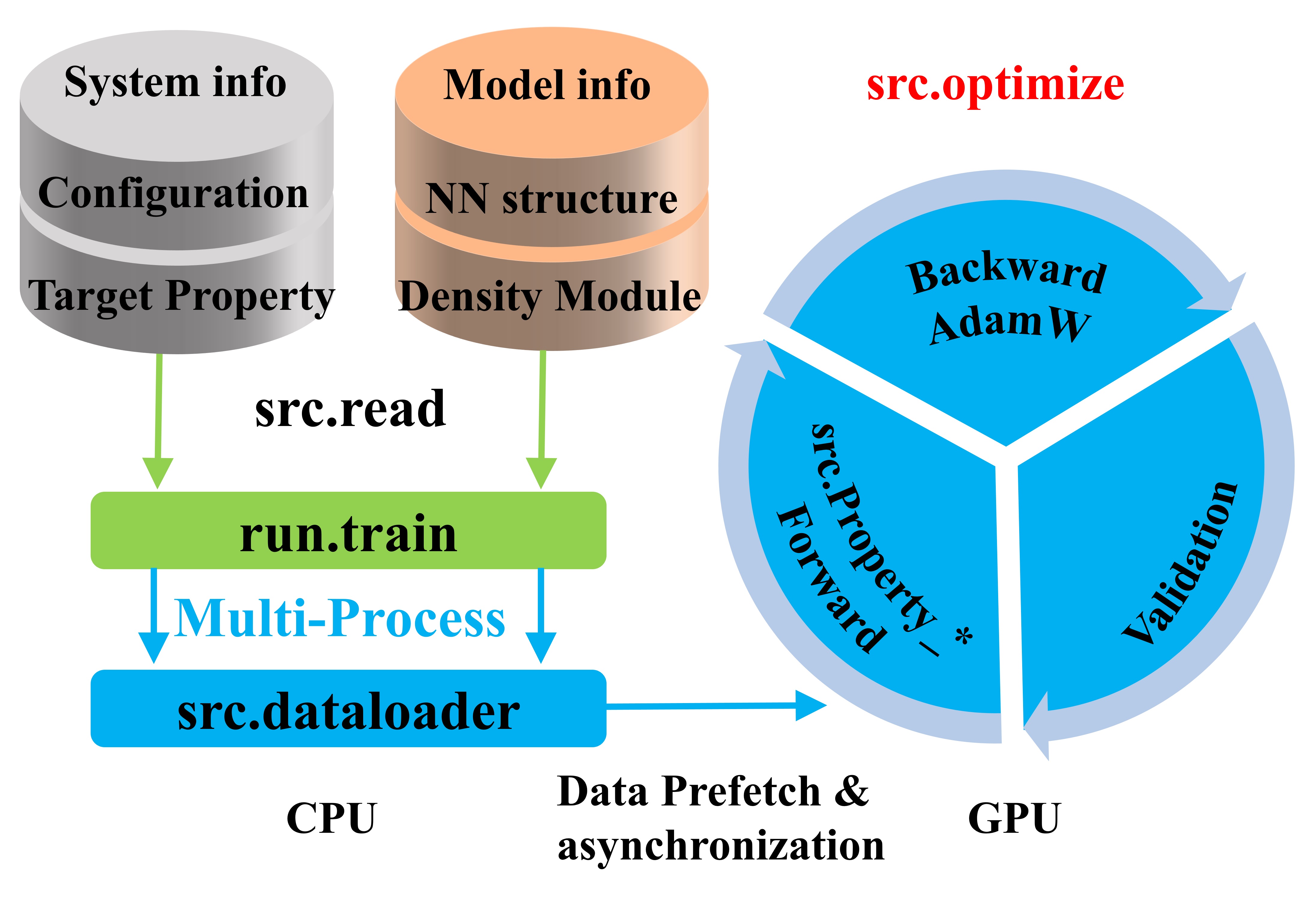
The training process can be divided into four parts: information loading, initialization, dataloader and optimization. First, the "src.read" will load the information about the systems and NN structures from the dataset and input files (“input_nn” and “input_density”) respectivrly. Second, the "run.train" module utilizes the loaded information to initialize various classes, including property calculator, dataloader, and optimizer. For each process, an additional thread will be activated in the "src.dataloader" module to prefetch data from CPU to GPU in an asynchronous manner. Meanwhile, the optimization will be activated in the "src.optimize" module once the first set of data is transferred to the GPU. During optimization, a learning rate scheduler, namely "ReduceLROnPlateau" provided by PyTorch, is used to decay the learning rate. Training is stopped when the learning rate drops below "end_lr" and the model that performs best on the validation set is saved for further investigation. 
Users can employ geometries, energies, atomic force vectors (or some other physical properties which are invariant under rigid translation, rotation, and permutation of identical atoms and their corresponding gradients) to construct a model. There are three routines to use this package:
The REANN Package is built based on PyTorch and uses the "opt_einsum" package for optimizing einsum-like expressions frequently used in the calculation of the embedded density. In order to run the REANN package, users need to install PyTorch (version: 2.0.0) based on the instructions on the PyTorch official site and the package named opt_einsum.
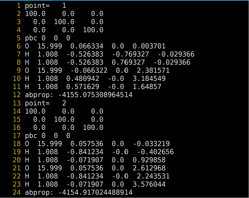
There are two directories that users need to prepare, namely, “train” and “val”, each of which includes a file “configuration” used to preserve the required information including lattice parameters, periodic boundary conditions, configurations, energy and atomic forces (if needed), dipole moments, polarizabilities, etc. For example, users want to represent the NMA system that has available atomic forces. The file "configuration" should be written in the following format. The first line can be an arbitrary character other than a blank line. The next three lines are the lattice vectors defining the unit cell of the system. The fifth line is used to enable(1)/disable(0) the periodic boundary conditions in each direction. In this example, NMA is not a periodic system, the fifth line should be “pbc 0 0 0”. For some gas-surface systems, only the x-y plane is periodic and the corresponding fifth line is “pbc 1 1 0”. Following N lines (N is the number of atoms in the system, here is 12): the columns from the left to right represent the atomic name, relative atomic mass, coordinates(x, y, z) of the geometry, atomic force vectors (if the force vector is not incorporated in the training, these three columns can be omitted). Next line: Start with "abprop:" and then follow bytarget property (energy/dipole/polzrizability). One example is stored in "data" folder.
In the section, we will introduce some hyparameters concerning the embedded density and NN structures that are essential for obtianing an exact representation. More detailed introduction of all parameters can be found on the manual in the "manual" floder. These parameters are set up in two files "input_nn" and "input_density" saved in the "para" floder of your work directory. one example of input_nn and input_density is placed in the "example" foleder.
- batchsize_train=64 # required parameters type: integer
- batchsize_val=128 # required parameters type: integer (Number of configurations used in each batch for train (batchsize_train) and validation (batchsize_val). Note, this "batchsize_train" is a key parameter concerned with efficiency. Normally, a large enough value is given to achieve high usage of the GPU and lead to higher efficiency in training if you have sufficient data. However, for small training data, a large "batchsize" can lead to a decrease in accuracy, probably owing to the decrease in the number of gradient descents during each epoch. The decrease in accuracy may be compensated by more epochs (increase the "patience_epoch" ) or a larger learning rate. Some detailed testing is required here to achieve a balance of accuracy and efficiency in training. The value of "batch_val" has no effect on accuracy, and thus a larger value is preferred.)
- oc_loop = 1 # type: integer (Number of iterations used to represent the orbital efficients.)
- cutoff = 4.5 # type: real number (Cutoff distances)
- nipsin= 2 # type: integer (Maximal angular momenta determine the orbital type (s, p, d ..))
- nwave=8 # type: integer (Number of radial Gaussian functions. This number should be a power of 2 for better efficiency.)
As mentioned earlier, the package interfaces with the LAMMPS framework by creating a new pair_style (fireann).MD simulations can be run in a multi-process or multi-threaded fashion on both GPUs and CPUs. MD simulations based on other MD packages such as i-pi can also be executed through the existing ipi-lammps interface. In addition, MD simulation can also be performed by the ASE interface. More details can be found in the manual.
In the “ASE” folder, there is a Python script named “ase_reann.py.”which serves as an example for calculating energy and atomic forces by utilizing the model saved in “PES.pt”. Note that the “atomtype” script used in the inference should match that found in the “input_density” file. In this interface, we do not use the default ASE neighbor list calculator. Instead, we employ a highly efficient Fortran implementation of a cell-linked algorithm to construct the neighbor list. To compile the Fortran code, f2py should be utilized, which generates a dynamic link library when executing the provided “run” script. This resulting dynamic link library can then be called by ASE or any Python-based evaluator.
If you use this package, please cite these works.
- The original EANN model: Yaolong Zhang, Ce Hu and Bin Jiang J. Phys. Chem. Lett. 10, 4962-4967 (2019).
- The EANN model for dipole/transition dipole/polarizability: Yaolong Zhang Sheng Ye, Jinxiao Zhang, Jun Jiang and Bin Jiang J. Phys. Chem. B 124, 7284–7290 (2020).
- The theory of REANN model: Yaolong Zhang, Junfan Xia and Bin Jiang Phys. Rev. Lett. 127, 156002 (2021).
- The details about the implementation of REANN: Yaolong Zhang, Junfan Xia and Bin Jiang J. Chem. Phys. 156, 114801 (2022).