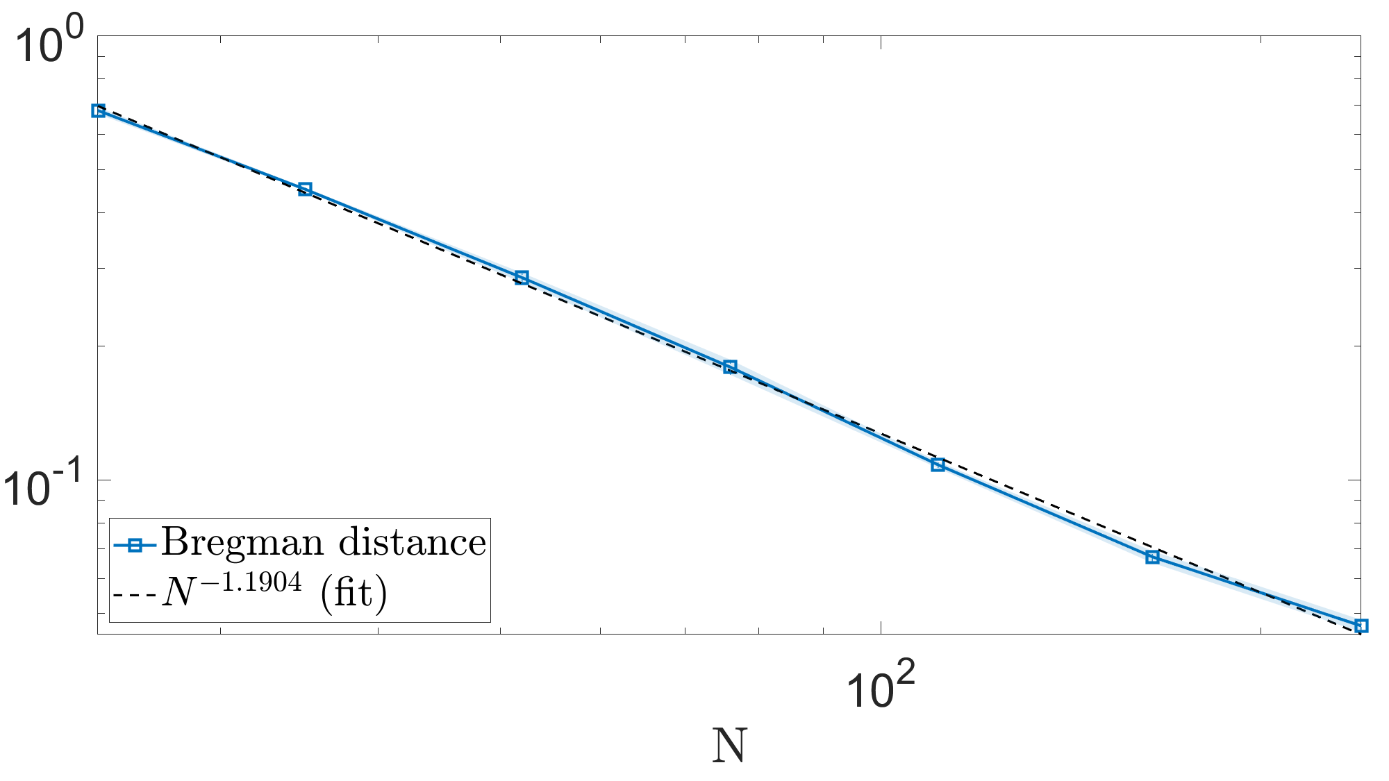
Numerical methods for estimating the Bregman distance decay rate using cylindrical shearlet regularization for dynamic tomography.

Figure: Example plot of Bregman error decay. Cylindrical shearlets and $p=\frac{3}{2}$-norm is used for regularization.

These algorithms are used to produce the numerical results in

T. A. Bubba, T. Heikkilä, D. Labate and L. Ratti,
"Regularization with optimal space-time priors",
arXiv pre-print: 2405.06337 (2024).

The references and necessary toolboxes are listed in the credits.

The repository contains the following files and folders.

root:

• Main_cylSh_VMILAn_cluster.m: the main function used to run the algorithm on different data, using different regularization methods (cylindrical shearlets or wavelets), noise models and parameters.

  Key parameters

  • dataset: either 'Stempo' or 'Cartoon'
  • p: $\ell^p$-norm used for regularization. p = 1 implemented separately and any p > 1 should in theory work but in practice only certain values (such as p = 1.5) are implemented.
  • transform: 1 for wavelets, 2 for cylindrical shearlets, (0 for identity or Tikhonov regularization: NOT IMPLEMENTED!)
  • c_alpha: regularization parameter. One value per setup is enough, it is automatically tuned for different N based on the theoretical decay rate.
  • fixed_noise: 0 for decreasing noise, i.e. noise magnitude and alpha decrease at rate $N^{-1}$; 1 for fixed noise, i.e. noise magnitude remains constant and alpha decreases at rate $N^{-1/3}$
  • Nsamp: number of samples per N, i.e. how many times each test is run with new realizations of noise and random projection angles.
  • Nangsamp, NangMin, NangMax: number of random projection angles N get chosen from a logarithmically spaced sequence of Nangsamp values, where NangMin is the minimum N and NangMax is the maximum N. If Nangsamp = 1, use N = NangMin.
  • c_delta: noise level. One value per setup is enough, it is automatically tuned for different N based on the theoretical rate.

  Other parameters

  • wname, level: change the wavelet family and decomposition level.
  • decomp, dsize, level: change the cylindrical shearlet parameters such as number of shearings, filter size and decomposition level.
  • opts. x0, obj, tolstop, stopcrit, scaling, savefreq: VMILA parameters for choosing starting point, "ground truth" for comparison, stopping tolerance, stopping criterion, option for adaptive bounds, how often iterates are stored.

• VMILAn_CTrandomAngles_l*_NNconstraint.m: function for calling the Variable Metric Inexact Line-search Algorithm (VMILA), p = 1 and p > 1 are implemented separately. Both use Non-Negativity constraint.

• SGP_VMILAn_CTrandomAngles_l*_NNconstraint.m: function for calling the Scaled Gradient Projection (SGP) algorithm to solve the dual problem during VMILA iteration, p = 1 and p > 1 are implemented separately. Both use Non-Negativity constraint.

• CreateFinalPlots_ErrorBar.m: function for generating the Bregman distance error plots used in the paper.

data:

• cartoonPhantom_256x256x*.mat: simulated phantom at twice the desired spatial resolution (256 x 256) and two temporal resolutions: T = 32 and T = 64. The data is simulated separately on the spot for the random projection angles.

• stempo/stempo_cwtRecn_280x280x16.mat: dynamic reconstruction from real tomography data using the STEMPO device. Regularized using 3D dual-tree complex wavelets.

• IMPORTANT: The STEMPO data is NOT included in the repostory since it can be found on Zenodo: 10.5281/zenodo.8239013. The stempo_seq8x180_2d_b8.mat data matches the 280x280x16 ground truth. See stempo.md for details.

plots: any plots created with CreateFinalPlots_ErrorBar.m are stored here.

tools:

• create_blkdiag_ct_operator_2d_*.m: functions for creating block-diagonal CT operators for different 2D geometries. These rely on the ASTRA Toolbox and HelTomo Toolbox.

• extrapolate*CtData.m: function for linearly extrapolating the random projections from real sinograms. There is a separate function for the STEMPO data.

• prepareRandomData.m: function for generating simulated data from a known phantom with twice the spatial resolution. No noise is added here!

• external.md: references to the external toolboxes necessary.

tools/util:

• SH2feas.m: project cylindrical shearlet coefficients (cell arrays) to the feasible region [-bound, bound].

• SHpnorm.m: computes the $\frac{1}{p} | U |_p^p$ function from the given cylindrical shearlet coefficients $U$ (cell array).

• cellnorm: computes the $\ell^p$-norm from the given cylindrical shearlet coefficients (cell array).

• SHsum.m: linear combination $aU + bV$ of cylindrical shearlet coefficients $U$ and $V$, scaled by $a$ and $b$.

• bregL1.m: symmetric Bregman distance $B(u,v)$ between $u$ and $v$, where $p=1$ and $Mu$, $Mv$ are the already decomposed inputs. $ B(u,v) = \langle sgn(Mu) - sgn(Mv), Mu - Mv \rangle$. This implementation matches the choice $\partial | \cdot | = sgn(\cdot)$ for the subdifferential.

• dec2waverec.m: helper function for setting the wavelet coefficients in to a struct for waverec3 to reconstruct.

• setup_cylindrical_filters: function for generating the cylindrical shearlet filters of desired size.

Original algorithm by Tatiana A. Bubba and Luca Ratti, used in

T. A. Bubba, M. Burger, T. Helin, and L. Ratti, "Convex regularization in statistical inverse learning problems", Inverse Problems and Imaging, 17, pp. 1193–1225 (2023).

T. A. Bubba and L. Ratti, "Shearlet-based regularization in statistical inverse learning with an application to x-ray tomography", Inverse Problems, p. 054001, (2022).

Adapted for dynamic tomography and 3D regularization by Tommi Heikkilä.

The minimization problem is solved with the Variable Metric Inexact Line-search Algorithm (VMILA) introduced in

S. Bonettini, I. Loris, F. Porta and M. Prato, "Variable metric inexact line-search based methods for nonsmooth optimization", SIAM J. Optim., 26 891–921, (2016).

The proximal operators require solving additional minimization problems. These are computed using the Scaled Gradient Projection (SGP) algorithm introduced in

S. Bonettini, R. Zanella and L. Zanni, "A scaled gradient projection method for constrained image deblurring", Inverse Problems 25 015002, (2006).

The 3D Discrete Wavelet Transform is part of the Wavelet Toolbox and the 3D cylindrical shearlets are based on

G. R. Easley, K. Guo, D. Labate and B. R. Pahari, "Optimally sparse representations of cartoon-like cylindrical data", The Journal of Geometric Analysis 31: 8926-8946, (2021).
https://github.com/tommheik/3d_cylind_shear

The tomography forward operator is computed using the ASTRA Toolbox

W. Van Aarle, W. J. Palenstijn, J. Cant, E. Janssens, F. Bleichrodt, A. Dabravolski, J. De Beenhouwer, K. J. Batenburg and J. Sijbers, "Fast and flexible x-ray tomography using the ASTRA toolbox", Opt. Express 24 25129–47 (2016).

W. Van Aarle, W. J. Palenstijn, J. De Beenhouwer, T. Altantzis, S. Bals, K. J. Batenburg and J. Sijbers, "The ASTRA toolbox: a platform for advanced algorithm development in electron tomography", Ultramicroscopy 157 35–47, (2015).

The algorithm also uses Spot and HelTomo

E. Van den Berg and M. P. Friedlander, "Spot - a linear-operator toolbox", v1.2, (2013) https://cs.ubc.ca/labs/scl/spot

A. Meaney, "HelTomo - Helsinki Tomography Toolbox", v2.0.0, (2022) https://github.com/Diagonalizable/HelTomo