An R package for analyzing scanpaths in eye movement data. The package includes a simple toy dataset and example code. Consult von der Malsburg & Vasishth (2011) for the details of this analysis method. The manual of the package can be found here and a PDF-version of this page here.
- [2021-07-09]
- Fixed a bug triggered when factors were used as trial identifiers.
- [2018-02-22]
- Added an interactive demo app that shows how the scanpath measure works.
- [2018-02-21]
- Added new functions
rscasimandplot_alignment. See section ’How the sausage is made’ below for details. Also note that the order of parameters forplot_scanpathshas changed for consistency with ggplot2. - [2018-02-20]
- The new default is no normalization of scasim scores. Improved documentation and examples for
find.fixationandmatch.scanpath. Minor improvement in functions for plotting scanpaths. - [2018-01-30]
- Version 1.06 doesn’t logarithmize fixation durations when calculating scanpath similarities. (In previous versions, when
normalize="durations"was used, the normalization was done using non-log-transformed durations, which could in some rare cases break the triangle inequality.)
To install the latest version of the package, execute the following commands:
library("devtools");
install_github("tmalsburg/scanpath/scanpath", dependencies=TRUE)The code shown below can also be found in the file README.R. Open that file in RStudio and play with it as you read through this mini-tutorial.
Let’s have a look at the toy data that is included in the package:
library(tidyverse)
library(magrittr)
library(scanpath)
data(eyemovements)
head(eyemovements)| subject | trial | word | x | y | duration |
|---|---|---|---|---|---|
| Anne | 1 | 1 | 46 | 384 | 319 |
| Anne | 1 | 3 | 131 | 388 | 147 |
| Anne | 1 | 2 | 106 | 386 | 88 |
| Anne | 1 | 3 | 165 | 387 | 156 |
| Anne | 1 | 4 | 186 | 386 | 244 |
| Anne | 1 | 5 | 264 | 388 | 193 |
To get a sense of what is going on in this data set, we create a series of plots. For this purpose, we use the function plot_scanpaths from the scanpath package. In the first plot below, each panel shows the data from one trial. There are three participants which are coded by color. The data is from a sentence reading task. The x-axis shows words and the y-axis time within trial in milliseconds.
plot_scanpaths(eyemovements, duration ~ word | trial, subject)We can see that the participants differ in their reading speed. Also we see that each participant read the sentence more or less straight from left to right (trials: 1, 4, 7), or with a short regressions from the end of the sentence to its beginning (trials: 2, 5, 8), or with a long regression from the end of the sentence (trials: 3, 6, 9).
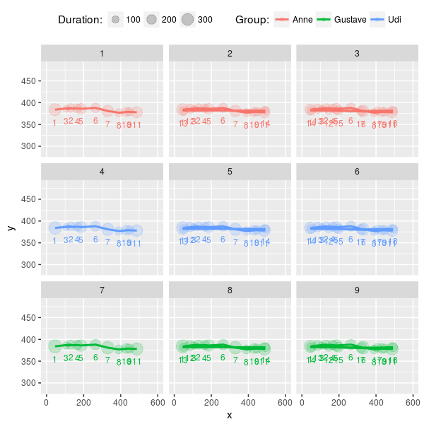
In the next plot, we use the fixations’ x- and y-coordinates. Each circle is a fixation and the size of the circle represents the duration of the corresponding fixation.
plot_scanpaths(eyemovements, duration ~ x + y | trial, subject)The function plot_scanpaths returns a ggplot object. This means that we add more elements to the plot before rendering. For example, we can labels the fixations with their index and change the limits of the axes:
plot_scanpaths(eyemovements, duration ~ x + y | trial, subject) +
  geom_text(aes(label=i), vjust=2.5, show.legend=FALSE, size=3) +
xlim(0, 600) + ylim(284, 484)In many analyses, it is not desirable to analyze the complete scanpaths as recorded during the experiment but to analyze some subset of the fixations. For instance, in a reading experiment, we might want to investigate how readers responded to a certain word and not care about what happened earlier. The scanpath package offers two functions that can be used to easily pinpoint and extract the fixations of interest: find.fixation and match.scanpath.
The function find.fixation identifies fixations that match a set of criteria which can be specified using regular expressions. For instance, the following code finds fixations on word 6:
idx <- find.fixation(eyemovements$word, eyemovements$trial, "6")
eyemovements[idx,]| subject | trial | word | x | y | duration |
|---|---|---|---|---|---|
| Anne | 1 | 6 | 330 | 381 | 290 |
| Anne | 2 | 6 | 330 | 381 | 290 |
| Anne | 3 | 6 | 330 | 381 | 290 |
| Anne | 3 | 6 | 320 | 381 | 189 |
| Udi | 4 | 6 | 330 | 381 | 319 |
| Udi | 5 | 6 | 330 | 381 | 319 |
| Udi | 6 | 6 | 330 | 381 | 319 |
| Udi | 6 | 6 | 320 | 381 | 208 |
| Gustave | 7 | 6 | 330 | 381 | 348 |
| Gustave | 8 | 6 | 330 | 381 | 348 |
| Gustave | 9 | 6 | 330 | 381 | 348 |
| Gustave | 9 | 6 | 320 | 381 | 227 |
Finding these fixations could also have been achieved with a subset operation. However, if have more complex criteria for the fixations we’re interested in, things can get rather tricky. For instance, a subset is not enough when we’re only interested in the second fixation on word 6 in each trial. The following code extracts only those:
idx <- find.fixation(eyemovements$word, eyemovements$trial, "6", nth=2)
eyemovements[idx,]| subject | trial | word | x | y | duration |
|---|---|---|---|---|---|
| Anne | 3 | 6 | 320 | 381 | 189 |
| Udi | 6 | 6 | 320 | 381 | 208 |
| Gustave | 9 | 6 | 320 | 381 | 227 |
Regular expressions also allow us to specify the context in which the fixations of interest appear. For instance the code below finds fixations on word 3 but only those that are followed by fixations on word 4:
idx <- find.fixation(eyemovements$word, eyemovements$trial, "34")
eyemovements[idx,]| subject | trial | word | x | y | duration |
|---|---|---|---|---|---|
| Anne | 1 | 3 | 165 | 387 | 156 |
| Anne | 2 | 3 | 165 | 387 | 156 |
| Anne | 3 | 3 | 165 | 387 | 156 |
| Udi | 4 | 3 | 165 | 387 | 172 |
| Udi | 5 | 3 | 165 | 387 | 172 |
| Udi | 6 | 3 | 165 | 387 | 172 |
| Gustave | 7 | 3 | 165 | 387 | 187 |
| Gustave | 8 | 3 | 165 | 387 | 187 |
| Gustave | 9 | 3 | 165 | 387 | 187 |
Here, we find fixations on word 3 that are preceded by fixations on word 1:
idx <- find.fixation(eyemovements$word, eyemovements$trial, "1(3)", subpattern=1)
eyemovements[idx,]| subject | trial | word | x | y | duration |
|---|---|---|---|---|---|
| Anne | 1 | 3 | 131 | 388 | 147 |
| Anne | 2 | 3 | 131 | 388 | 147 |
| Anne | 3 | 3 | 131 | 388 | 147 |
| Udi | 4 | 3 | 131 | 388 | 162 |
| Udi | 5 | 3 | 131 | 388 | 162 |
| Udi | 6 | 3 | 131 | 388 | 162 |
| Gustave | 7 | 3 | 131 | 388 | 176 |
| Gustave | 8 | 3 | 131 | 388 | 176 |
| Gustave | 9 | 3 | 131 | 388 | 176 |
The following code finds fixations on the last word but only of those that are not directly preceded by fixations on words 4 to 7:
idx <- find.fixation(eyemovements$word, eyemovements$trial, "[^4-7](8)", subpattern=1)
eyemovements[idx,]| subject | trial | word | x | y | duration |
|---|---|---|---|---|---|
| Anne | 2 | 8 | 492 | 382 | 143 |
| Udi | 5 | 8 | 492 | 382 | 157 |
| Gustave | 8 | 8 | 492 | 382 | 172 |
The function match.scanpath works similarly but can be used to identify not just individual fixations but sequences of fixations (let’s call them scanpathlets). For example, the following code finds scanpathslets spanning words 6, 7, and 8 but only those that directly preceded by a fixation on word 4:
idx <- match.scanpath(eyemovements$word, eyemovements$trial, "4([678]+)", subpattern=1)
scanpathlets <- eyemovements[idx,]
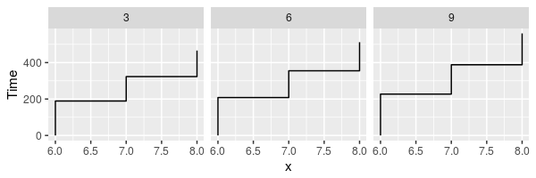
plot_scanpaths(scanpathlets, duration~word|trial)
See the documentation of find.fixation and match.scanpath for more details and examples.
Next, we calculate the pair-wise similarities of the nine scanpaths in the dataset using the scasim measure. A simplifying intuition is that the measure quantifies the time that was spent looking at different things (or at the same things but in different order). For a precise definition see von der Malsburg & Vasishth (2011).
d1 <- scasim(eyemovements, duration ~ x + y | trial, 512, 384, 60, 1/30)
round(d1)| 1 | 2 | 3 | 4 | 5 | 6 | 7 | 8 | 9 | |
|---|---|---|---|---|---|---|---|---|---|
| 1 | 0 | 454 | 1129 | 217 | 717 | 1395 | 435 | 980 | 1670 |
| 2 | 454 | 0 | 675 | 671 | 263 | 941 | 889 | 526 | 1216 |
| 3 | 1129 | 675 | 0 | 1346 | 938 | 320 | 1564 | 1201 | 641 |
| 4 | 217 | 671 | 1346 | 0 | 500 | 1242 | 218 | 763 | 1509 |
| 5 | 717 | 263 | 938 | 500 | 0 | 742 | 718 | 263 | 1009 |
| 6 | 1395 | 941 | 320 | 1242 | 742 | 0 | 1460 | 1005 | 321 |
| 7 | 435 | 889 | 1564 | 218 | 718 | 1460 | 0 | 545 | 1355 |
| 8 | 980 | 526 | 1201 | 763 | 263 | 1005 | 545 | 0 | 810 |
| 9 | 1670 | 1216 | 641 | 1509 | 1009 | 321 | 1355 | 810 | 0 |
Like the function plot_scanpaths, the function scasim takes a data frame and a formula as parameters. The formula specifies which columns in the data frame should be used for the calculations. To account for distortion due to visual perspective, the comparison of the scanpaths is carried out in visual field coordinates (latitude and longitude). In order to transform the pixel coordinates provided by the eye-tracker to visual field coordinates, the scasim function needs some extra information. The first is the position of the gaze when the participant looked straight ahead (512, 384, in the present case), the distance of the eyes from the screen (60 cm), and the size of one pixel in the unit that was used to specify the distance from the screen (1/30). Finally, we have to specify a normalization procedure. normalize=FALSE means that we don’t want to normalize. See the documentation of the scasim function for details.
The time that was spent looking at different things of course depends on the duration of the two compared trials. (total duration of the two compared scanpaths constitutes an upper bound). This means that two long scanpaths may have a larger dissimilarity than two shorter scanpaths even if they look more similar. Depending on the research question, this may be undesirable. One way to get rid of the trivial influence of total duration is to normalize the dissimilarity scores. For example, we can divide them by the total duration of the two compared scanpaths:
d2 <- scasim(eyemovements, duration ~ x + y | trial, 512, 384, 60, 1/30,
             normalize="durations")
round(d2*100)| 1 | 2 | 3 | 4 | 5 | 6 | 7 | 8 | 9 | |
|---|---|---|---|---|---|---|---|---|---|
| 1 | 0 | 9 | 21 | 5 | 14 | 25 | 9 | 18 | 28 |
| 2 | 9 | 0 | 12 | 13 | 5 | 15 | 17 | 9 | 19 |
| 3 | 21 | 12 | 0 | 24 | 15 | 5 | 27 | 19 | 9 |
| 4 | 5 | 13 | 24 | 0 | 9 | 21 | 4 | 14 | 24 |
| 5 | 14 | 5 | 15 | 9 | 0 | 12 | 13 | 4 | 15 |
| 6 | 25 | 15 | 5 | 21 | 12 | 0 | 24 | 15 | 4 |
| 7 | 9 | 17 | 27 | 4 | 13 | 24 | 0 | 9 | 21 |
| 8 | 18 | 9 | 19 | 14 | 4 | 15 | 9 | 0 | 12 |
| 9 | 28 | 19 | 9 | 24 | 15 | 4 | 21 | 12 | 0 |
The number are smaller now and can be interpreted as the percentage of time that was spent looking at different things.
The numbers in the matrix above capture a lot of information about the scanpath variance in the data set. However, dissimilarity scores are somewhat tricky to analyze. One problem is that these values have strong statistical dependencies. When we change one scanpath, this affects n dissimilarity scores. This has to be kept in mind when doing inferential stats directly on the dissimilarity scores. While there are solutions for this, it is typically more convenient to produce a representation of scanpath variance that is free from this problem. One such representation is what we call the “map of scanpath space.” On such a map, every point represents a scanpath and the distances on the map reflect the dissimilarities according to our scanpath measure, i.e. the dissimilarity scores in the matrix above.
The method for calculating these maps is called multi-dimensional scaling and one simple version of the general idea is implemented in the function cmdscale (see also isoMDS in the MASS package).
map <- cmdscale(d2)
round(map, 2)| V1 | V2 | |
|---|---|---|
| 1 | -0.12 | -0.07 |
| 2 | -0.01 | -0.06 |
| 3 | 0.12 | -0.08 |
| 4 | -0.11 | 0 |
| 5 | -0.01 | 0.01 |
| 6 | 0.12 | 0 |
| 7 | -0.11 | 0.07 |
| 8 | 0 | 0.07 |
| 9 | 0.13 | 0.07 |
The table above contains two numbers for each scanpath in the data set. These numbers (V1 and V2) determine a scanpath’s location in the two-dimensional scanpath space created by cmdscale. How many dimensions we need is an empirical question.
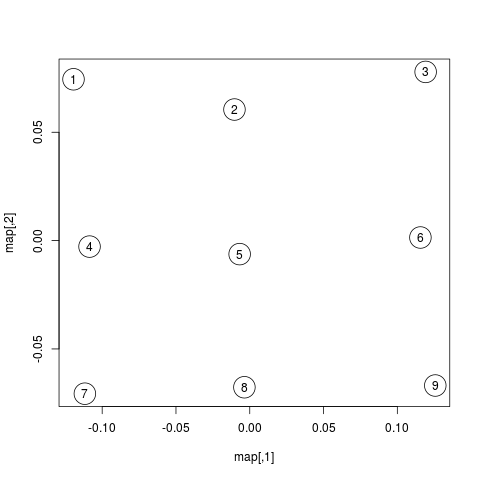
Below is a plot showing the map of scanpaths:
map <- map %*% matrix(c(1, 0, 0, -1), 2)  # flip y-axis
plot(map, cex=4)
text(map, labels=rownames(map))
Interestingly, the scanpaths are arranged in the same way as in the plot of the data at the top. Participants are arranged vertically and reading patterns are horizontally. This suggests that scasim not just recovered these two different kinds of information (reading speed and reading strategy) but also that it can distinguish between them.
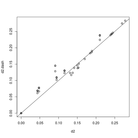
To test how well this map represents the original dissimilarity scores, we can calculate the pair-wise differences on the map and compare them to the pair-wise scasim scores:
d2.dash <- as.matrix(dist(map))
plot(d2, d2.dash)
abline(0, 1)
This plot suggests that the map preserves the variance in dissimilarity scores really well. Given this very good fit of the map, it appears that two dimensions were sufficient to describe the scanpath variance that is captured by scasim. This is not surprising because the scanpaths in the toy data set were designed to vary with respect to two properties: 1.) The speed of the reader, and 2.) whether there was a regression back to the beginning of the sentence and how long it was.
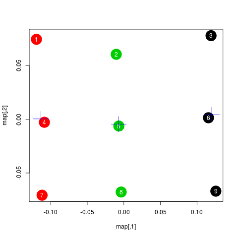
The benefit of the map representation is that it has much weaker statistical dependencies and that it is much more suitable for all kinds of analyses. For example, we can choose among a large number of clustering algorithms to test whether there are groups of similar scanpaths in a data set. Below, we use the simple k-means algorithm to illustrate this:
set.seed(4)
clusters <- kmeans(map, 3, iter.max=100)
plot(map, cex=4, col=clusters$cluster, pch=19)
text(map, labels=rownames(map), col="white")
points(clusters$centers, col="blue", pch=3, cex=4)
In this plot, color indicates to which cluster a scanpath belongs and the crosses show the center of each cluster. We see that the clusters correspond to the different reading patterns and that participants are ordered according to their reading speed within the clusters.
Apart from cluster analyses there are many other ways to analyze scanpath variance. See the articles listed below for more details.
For educational purposes, the package also includes a pure-R implementation of the scasim measure in the form of the function rscasim. This function calculates the similarity of two scanpaths and returns the alignment of fixations obtained with the Needleman-Wunsch algorithm.
s <- subset(eyemovements, trial==1)
t <- subset(eyemovements, trial==9)
alignment <- rscasim(s, t, duration ~ x + y | trial,
                     512, 384, 60, 1/30)
round(alignment)| s | t | cost |
|---|---|---|
| 1 | 1 | 4 |
| 2 | 2 | 29 |
| 3 | 3 | 18 |
| 4 | 4 | 31 |
| 5 | 5 | 49 |
| 6 | 6 | 39 |
| 7 | 7 | 58 |
| 8 | 8 | 28 |
| 9 | 9 | 30 |
| 10 | 10 | 34 |
| 11 | 11 | 55 |
| NA | 12 | 146 |
| NA | 13 | 222 |
| NA | 14 | 151 |
| NA | 15 | 216 |
| NA | 16 | 227 |
| NA | 17 | 161 |
| NA | 18 | 172 |
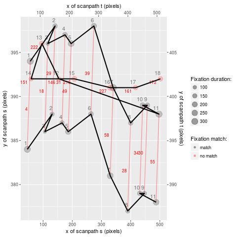
Each row in the table above describes one edit operation. The columns s and t contain the indices of the fixations involved in the edit and the column cost shows the cost of the edit. The sum of the values in the cost column is the total dissimilarity of the two scanpaths.
If both s and t contain an index, this means that two fixations were matched. If either column contains an NA, that means that a fixation in one scanpath had no matching counterpart in the other scanpath. The alignment can be visualized with the function plot_alignment:
plot_alignment(s, t, alignment, duration ~ x + y | trial, 10, 10)- von der Malsburg, T., & Vasishth, S. (2011). What is the scanpath signature of syntactic reanalysis? Journal of Memory and Language, 65(2), 109–127. https://dx.doi.org/10.1016/j.jml.2011.02.004
- von der Malsburg, T., Kliegl, R., & Vasishth, S. (2015). Determinants of scanpath regularity in reading. Cognitive Science, 39(7), 1675–1703. https://dx.doi.org/10.1111/cogs.12208
- von der Malsburg, T., & Vasishth, S. (2013). Scanpaths reveal syntactic underspecification and reanalysis strategies. Language and Cognitive Processes, 28(10), 1545–1578. https://dx.doi.org/10.1080/01690965.2012.728232
- von der Malsburg, T., Vasishth, S., & Kliegl, R. (2012). Scanpaths in reading are informative about sentence processing. In P. B. Michael Carl, & K. K. Choudhary, Proceedings of the First Workshop on Eye-tracking and Natural Language Processing (pp. 37–53). Mumbai, India: The COLING 2012 organizing committee. https://tmalsburg.github.io/MalsburgEtAl2012Coling.pdf
- Parshina, O., Sekerina, I., Lopukhina, A., & von der Malsburg, Titus (2022). Monolingual and bilingual reading strategies in Russian: An exploratory scanpath analysis. Reading Research Quarterly, 57(2). https://dx.doi.org/10.1002/rrq.414


