Welcome to our BayesFlow library for efficient simulation-based Bayesian workflows! Our library enables users to create specialized neural networks for amortized Bayesian inference, which repays users with rapid and fully Bayesian parameter estimation or model comparison after a simulation-based training phase.

For starters, check out some of our walk-through notebooks:

1. Basic amortized posterior estimation
2. Intermediate posterior estimation
3. Posterior estimation for ODEs

The project documentation is available at http:https://bayesflow.readthedocs.io

A cornerstone idea of amortized Bayesian inference is to employ generative neural networks for parameter estimation, model comparison, and model validation when working with intractable simulators whose behavior as a whole is too complex to be described analytically. The figure below presents a higher-level overview of neurally bootstrapped Bayesian inference.

The core functionality of BayesFlow is amortized Bayesian posterior estimation, as described in our paper:

Radev, S. T., Mertens, U. K., Voss, A., Ardizzone, L., & Köthe, U. (2020). BayesFlow: Learning complex stochastic models with invertible neural networks. IEEE Transactions on Neural Networks and Learning Systems, available for free at: https://arxiv.org/abs/2003.06281.

However, since then, we have substantially extended the BayesFlow library such that it is now much more general and cleaner than what we describe in the above paper.

import numpy as np
import bayesflow as bf

To introduce you to the basic workflow of the library, let's consider a simple 2D Gaussian model, from which we want to obtain posterior inference. We assume a Gaussian simulator (likelihood) and a Gaussian prior for the means of the two components, which are our only model parameters in this example:

def simulator(theta, n_obs=50, scale=1.0):
    return np.random.default_rng().normal(loc=theta, scale=scale, size=(n_obs, theta.shape[0]))
    
def prior(D=2, mu=0., sigma=1.0):
    return np.random.default_rng().normal(loc=mu, scale=sigma, size=D)

Then, we connect the prior with the simulator using a GenerativeModel wrapper:

generative_model = bf.simulation.GenerativeModel(prior, simulator)

Next, we create our BayesFlow setup consisting of a summary and an inference network:

summary_net = bf.networks.InvariantNetwork()
inference_net = bf.networks.InvertibleNetwork(num_params=2)
amortizer = bf.amortizers.AmortizedPosterior(inference_net, summary_net)

Finally, we connect the networks with the generative model via a Trainer instance:

trainer = bf.trainers.Trainer(amortizer=amortizer, generative_model=generative_model)

We are now ready to train an amortized posterior approximator. For instance, to run online training, we simply call:

losses = trainer.train_online(epochs=10, iterations_per_epoch=500, batch_size=32)

Before inference, we can use simulation-based calibration (SBC, https://arxiv.org/abs/1804.06788) to check the computational faithfulness of the model-amortizer combination:

fig = trainer.diagnose_sbc_histograms()

The histograms are roughly uniform and lie within the expected range for well-calibrated inference algorithms as indicated by the shaded gray areas. Accordingly, our amortizer seems to have converged to the intended target.

Amortized inference on new (real or simulated) data is then easy and fast. For example, we can simulate 200 new data sets and generate 500 posterior draws per data set:

new_sims = trainer.configurator(generative_model(200))
posterior_draws = amortizer.sample(new_sims, n_samples=500)

We can then quickly inspect the how well the model can recover its parameters across the simulated data sets.

fig = bf.diagnostics.plot_recovery(posterior_draws, new_sims['parameters'])

For any individual data set, we can also compare the parameters' posteriors with their corresponding priors:

fig = bf.diagnostics.plot_posterior_2d(posterior_draws[0], prior=generative_model.prior)

We see clearly how the posterior shrinks relative to the prior for both model parameters as a result of conditioning on the data.

• Radev, S. T., Mertens, U. K., Voss, A., Ardizzone, L., & Köthe, U. (2020). BayesFlow: Learning complex stochastic models with invertible neural networks. IEEE Transactions on Neural Networks and Learning Systems, available for free at: https://arxiv.org/abs/2003.06281.

• Radev, S. T., Graw, F., Chen, S., Mutters, N. T., Eichel, V. M., Bärnighausen, T., & Köthe, U. (2021). OutbreakFlow: Model-based Bayesian inference of disease outbreak dynamics with invertible neural networks and its application to the COVID-19 pandemics in Germany. PLoS computational biology, 17(10), e1009472.

• von Krause, M., Radev, S. T., & Voss, A. (2022). Mental speed is high until age 60 as revealed by analysis of over a million participants. Nature Human Behaviour, 6(5), 700-708.

What if we are dealing with misspecified models? That is, how faithful is our amortized inference if the generative model is a poor representation of reality? A modified loss function optimizes the learned summary statistics towards a unit Gaussian and reliably detects model misspecification during inference time.

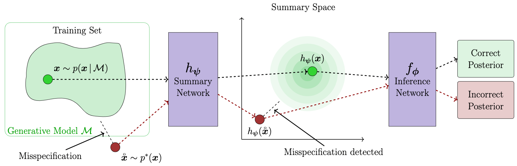
In order to use this method, you should only provide the summary_loss_fun argument to the AmortizedPosterior instance:

amortizer = bf.amortizers.AmortizedPosterior(inference_net, summary_net, summary_loss_fun='MMD')

The amortizer knows how to combine its losses.

• Schmitt, M., Bürkner P. C., Köthe U., & Radev S. T. (2022). Detecting Model Misspecification in Amortized Bayesian Inference with Neural Networks. ArXiv preprint, available for free at: https://arxiv.org/abs/2112.08866

Example coming soon...

• Radev S. T., D’Alessandro M., Mertens U. K., Voss A., Köthe U., & Bürkner P. C. (2021). Amortized Bayesian Model Comparison with Evidental Deep Learning. IEEE Transactions on Neural Networks and Learning Systems. doi:10.1109/TNNLS.2021.3124052 available for free at: https://arxiv.org/abs/2004.10629

Example coming soon...