1. Chapter 1: Reliable, Scalable, and Maintainable Applications
2. Chapter 2: Data Model and Query Languages
3. Chapter 3: Storage and retrieval
4. Chapter 4: Encoding and Evolution
5. Chapter 5: Replication
6. Chapter 6: Partitioning
7. Chapter 7: Transactions
8. Chapter 8: The Trouble with Distributed Systems
9. Chapter 9: Consistency and Consensus
10. Chapter 10: Batch Processing
11. Chapter 11: Stream Processing

We call an application data-intensive if data is its primary challenge - the quantity of data, the complexity of data, or the speed at which it is changing - as opposed to compute-intensive, where CPU cycles are the bottleneck.

• A data-intensive application is typically built from standard building blocks that provide commonly needed functionality. Many applications need to:
  • Store data so that they, or another application, can find it again later (databases)
  • Remember the result of an expensive operation, to speed up reads (caches)
  • Allow users to search data by keyword or filter it in various ways (search indexes)
  • Send a message to another process, to be handled asynchronously (stream processing)
  • Periodically crunch a large amount of accumulated data (batch processing)

Although a database and a message queue have some superficial similarity - both store data for some time - they have very different access patterns, which means different characterstics, and thus very different implementation.

There are datastores that are also used as message queues (Redis), and there are message queues with database-like durability guarantees (Apache Kafka).

If you have an application-managed caching layer (using Memcached or similar), or a full-text search server (such as Elasticsearch or Solr) separate from your main database, it is normally the application code’s responsibility to keep those caches and indexes in sync with the main database.

Stitching smaller systems together results in a larger data system, with different characteristics.

Figure 1-1 One possible architecture for a data system that combines several components.

We focus on three concerns that are important in most software systems:

• Reliability: The system should work correctly (performing the correct function at the desired level of performance) even in the face of adversity.
• Scalability: As the system grows(in data , traffic volume, or complexity), there should be reasonable ways of dealing with that growth.
• Maintainability: People should be able to work on the system productively in the future.

• Continue to work when faults (NOT failure!) occur. We say such a system is fault-tolerant.
• Faults is defined as components of the system deviating from the spec while failure is defined as a system stop working entirely.
• It is impossible to reduce faults to 0; therefore, we should design a system that tolerates faults.
• Introducing random faults (as in Netflix Chaos Monkey) could improve confidence in fault tolerant systems.
• For security issues, we would prefer to prevent faults over tolerating them, as security breaches cannot be cured.

• In the past, people use redundant hardware to keep machine/service running.
• Hard disks are reported as having a mean time to failure (MTTF) of about 10 to 50 years. Thus, on a storage cluster with 10,000 disks, we should expect on average one disk to die per day.
• AWS’s virtual machine platforms are designed to prioritize flexibility and elasticity over single-machine reliability.
• Recently, platforms are designed to prioritize flexibility and elasticity. Systems can tolerate loss of whole machines. No down time scheduled needed for single machine maintenance.

• Software errors/bugs are more systematic. They impact all machines in the same service.
• Alerts can help check the SLA guarantees.

• Most outages are human errors. We can
  • Minimize opportunities for errors through designs.
  • Decouple where mistakes are made (sandbox) and where the mistakes causes failures (production).
  • Test thoroughly, including unit, integration, and manual tests.
  • Allow quick and easy recovery to minimize impact.
  • Set up clear monitoring on performance metrics and error rates.

• Reliability is important for the business. Any down time could be revenue losses.
• There are situations where we may tradeoff reliability for lower development cost, but we should be very conscious when we are cutting corners.

• Scalability is the term we use to describe a system’s ability to cope with increased load.

• Described with load parameters, which has different meaning under different architectures. It can be requests per second for services, read write ratio for databases, number of simultaneous users. Sometimes the average case matters, and sometimes the bottleneck is dominated by a few extreme cases.

• Twitter example

  • Twitter has two main operations: post Tweet and home timeline (~100x more requests than post Tweet).
  • Approach 1: If we store Tweets in a simple database, home timeline queries may be slow. Posting a tweet simply inserts the new tweet into a global collection of tweets. When a user requests their home timeline, look up all the people they follow, find all the tweets for each of those users, and merge them.
  • Approach 2: We can push Tweets into the home timeline cache of each follower when a Tweet is published. Maintain a cache for each user’s home timeline — like a mailbox of tweets for each recipient user. When a user posts a tweet, look up all the people who follow that user, and insert the new tweet into each of their home timeline caches.
  • Approach 2 does not work for users with many followers, since the approach would need to update too many home timeline caches.
  • Distribution of followers in this case is a load parameter.
  • We can use approach 1 for users with many followers and approach 2 for the others.
  • Twitter is now implementing a hybrid of both approaches. For most users, tweets continue to be fanned out to home timelines at the time when they are posted. However, for a small number of users with millions of followers (celebrities), they are exempted from the fan out.

• Two ways to look at performance.
  • When we increase load parameters and keep resources unchanged. How is the performance affected.
  • When we increase load parameters how much resource do we need to keep performance unchanged.
• Batch processing systems cares about throughput (number of records processed per second).
• Online systems cares about the response time, which is measured in percentiles like p50, p90, p99, p999.
• Random additional latency could be introduced by a context switch to a background process, the loss of a network packet and TCP retransmission, a garbage collection pause, a page fault forcing a read from disk, mechanical vibrations in the server rack, or many other causes.
• Tail latencies (p999) are sometimes important as they are usually requests from users with a lot of data.
• Percentiles are often used in service level objectives (SLOs) and service level agreements (SLAs)
• Queuing delays often account for a large part of high percentiles. Since parallelism is limited in servers. Slow requests may cause head-of-line blocking and make subsequent requests slow.
• The latency from an end user request is the slowest of all the parallel calls. The more backend calls we make, the higher the chance that one of the requests were slow. This is known as tail latency amplification.

• Scaling up (vertical scaling, with a more powerful machine) and scaling out (horizontal scaling, distributing the load across multiple machines, the shared-nothing architecture) are two popular approaches to cope with increasing load. Good architectures usually involves a mixture of both.
• Elastic systems can add computing resources when load increases automatically but it may have more surprises.
• Scaling up stateful data systems can be complex. For this reason, common wisdom is to use a single node until cost or availability requirements are no longer satisfied. Of course this may change in the future.
• The architecture for large scale systems is usually highly specific and built around its assumptions on which operations will be common or rare. There is no one-size-fits-all scalable architecture.

• Three design principles to minimize pain for maintenance.

• Operations are for keeping a software system running smoothly.
• Good operability means making routine tasks easy. Data systems can
  • Provide visibility into the runtime behavior
  • Provide support for automation and integration with standard tools
  • Avoid dependencies on individual machines
  • Provide good documentation
  • Provide good default behavior
  • Self-healing where appropriate
  • Minimize surprises

• Complexity slows down engineers working on the system and increases the cost of maintenance.
• Possible complexity symptoms: explosion of state space, tight coupling of modules, tangled dependencies, inconsistent naming and terminology, hacks for solving performance problems, special cases for workarounds, etc.
• We can remove accidental complexity, which is complexity not inherent in the business problem. This can be done through abstraction and hiding implementation details.

• System requirements will change so we need to make making changes easy.

• Test-driven development and refactoring are tools for building software that is easier to change.

• Refactoring large data systems is different from refactoring a small local application (Agile); therefore, we use the term evolvability to refer to ease to make changes in a data system.

• Functional requirements: what the application should do

• Nonfunctional requirements: general properties like security, reliability, compliance, scalability, compatibility and maintainability.

• Data models are important part of developing software, it deeply affects how we think about the problem.
• Data models are built by layering one on top of another. The key question is: “how is it represented in terms of the next-lower layer?” Each layer hides the complexity of the layers below by providing a clean model.
• The data model has a profound effect on what the software above can or cannot do.
• In this chapter, we will compare the relational model, the document model, and a few graph-based models. We will also look at and compare various query languages.

• The goal of the relational model is to hide implementation details behind a clean interface.
• SQL was rooted in relational databases for business data processing in the 1960s and 1970s, and was used for transaction processing and batch processing.
• SQL was proposed in 1970 and is probably the best-known data model, where data is organized into relations (tables), which is an unordered collection of tuples (rows).

• NoSQL was just a catchy hashtag on Twitter for a meetup. NoSQL is the latest attempt to overthrow the relational model’s dominance.
• Driving forces for NoSQL
  • A need for better scalability (larger datasets, high write throughput)
  • Preference for free and open source software
  • Specialized query operations that are not supported by the relational model
  • The restrictiveness of the relational schemas
• It’s likely that relational databases will continue to be used along with many nonrelational databases.

• With a SQL model, if data is stored in a relational tables, an awkward translation layer is translated, this is called impedance mismatch.
• Strategies to deal with the mismatch
  • Normalized databases with foreign keys.
  • Use a database that Supports for structured data (PostgreSQL)
  • Encode as JSON or XML and store as text in database. It can’t be queried this way.
  • Store as JSON in a document in document-oriented databases (MongoDB). This has a better locality than the normalized representation.
• JSON representation has better locality than the multi-table SQL schema. All the relevant information is in one place, and one query is sufficient.

• For enum-type strings, we can store a separate normalized ID to string table, and use the ID in other parts of the database. This will enforce consistency (same spelling, better search), avoid ambiguity, be easier to update, support localization.
• Using ids reduces duplication. This is the key idea behind normalizing databases. Yet this requires a many-to-one relationship, which may not work well with document databases, whose support for joins are weak.

• We then compare the data model of relational and document databases.
  • Document databases: better schema flexibility, better performance due to locality, and closer to data structures in applications.
  • Relational databases: better support for joins, and many-to-one and many-to-many relationships.

• Document model may be a good choice if the application has a document-like structure:tree of one-to-many relationships, while relational models may require splitting a document-like structure into multiple tables.
• Records in document models are more difficult to directly access when they are deeply nested.
• For applications with many-to-many relationships, document models are less appealing due to the poor support for joins.
• For highly interconnected data, document model is awkward, and the relational model is acceptable, and graph models are the most natural.

• XML support in relational databases usually comes with schema validation while JSON support does not.
• Document databases are sometimes called schemaless, yet there is an implicit schema. A more accurate term is schema-on-read, meaning schema is only interpreted when data is read, in contrast with schema-on-write for relational database, where validation occurs during write time.
• An analogy to type checking is dynamic type checking (runtime) and static typing checking (compile-time). In general there is no right or wrong answer.
• To change a schema in document databases, applications would start writing new documents with the new schema, while in relational databases, one would need a migration query (which is quick for most databases, except MySQL).
• Schema-on-read is advantageous if items in the collection don’t all have the same structure.
• Schema-on-write is advantageous when all records are expected to have the same structure.

• If the whole document (string of JSON, XML) is required by application often, there is a performance advantage to this storage locality (single lookup, no joins required). If only a small portion of the data is required, this can be wasteful.
• It’s generally recommended to keep documents small and avoid writes that increases the size of documents (same size updates can be done in-place).
• Google’s Spanner database allows table rows to be nested in a parent table. Oracle’s database allows multi-table index cluster tables. The column-family concept (used in Cassandra and HBase) has a similar purpose for managing locality.

• Most relational databases (except MySQL) supports XML. PostgreSQL, MySQL, DB2 supports JSON.
• RethinkDQ supports joins, and some MongoDB drivers resolves database references.
• A hybrid of relational and document models is probably the future.

• SQL is a declarative query language.
• In a declarative language, only the goal is specified, not how the goal is achieved. It hides implementation details and leaves room for performance optimization.
• The fact that SQL is more limited in functionality gives databases more room for automatic optimizations.
• Declarative code is easier to parallelize as execution order is not specified.

• CSS and XML are declarative languages to specify styling in HTML, while changing styles directly through Javascript is imperative.
• Specifying styles using CSS is much better than changing styles directly using Javascript.

• MapReduce is a programming model for processing large amounts of data in bulk across many machines, and a limited form of MapReduce is supported by MongoDB and CouchDB.
• MapReduce is somewhere between declarative and imperative.
• SQL can, but not necessarily have to, be implemented by MapReduce operations.
• MongoDB supports a declarative query language called aggregation pipeline, where users don’t need to coordinate a map and reduce function themselves.

• An application with mostly one-to-many relationships or no relationships between records, the document model is appropriate, but for many-to-many relationships, graph models are more appropriate.
• Graphs can be homogeneous, where all vertices represent the same type of object and heterogeneous, where vertices may represent completely different objects.

• In the property graph model, each vertex consists of
  • A unique identifier
  • A set of outgoing edges
  • A set of incoming edges
  • A collection of properties (key-value pairs)
• Each edge consists of
  • A unique identifier
  • The vertex at which the edge starts (the tail vertex)
  • The vertex at which the edge ends (the head vertex)
  • A collection of properties (key-value pairs)
• The property graph model is analogous to storing two relational databases, one for vertices, one for edges.
• Multiple relationships can be stored within the same graph by proper labeling the edges.
• Graphs can be easily extended to accommodate new data types.

• Cypher is a declarative query language for property graphs, created for the Neo4j graph database.

• Usually, we know which joins to run in relational database queries, yet in a graph query, the number of joins is not fixed in advance, as we may need to follow an edge multiple times.

• In a triple-store, all information is stored in a three-part statement: subject, predicate, object.
• The subject is equivalent to a vertex in a graph.
• The object can be:
  • A value in a primitive datatype. In this case, the predicate and object forms the key and value of a property of the subject vertex.
  • Another vertex in the graph. In this case, the predicate is the edge between the subject vertex and the object vertex.

• Databases fundamentally does two things: Store data and retrieve the stored data.
• Chapter 3 discusses how data model and queries are interpreted by databases.
• Understanding under-the-hood details can help us pick the right solution and tune the performance.
• We’ll first look at two types of storage engines: log-structured and page-oriented storage engines.

• Many databases internally uses a log, which is a append-only data file.
• To retrieve data efficiently, we need an index, which is an additional structure derived from primary data and only affects performance of queries.
• Well-chosen indexes speed up queries but slow down writes. Therefore, databases don’t index everything by default and requires developers to use knowledge of query pattens to choose index manually.

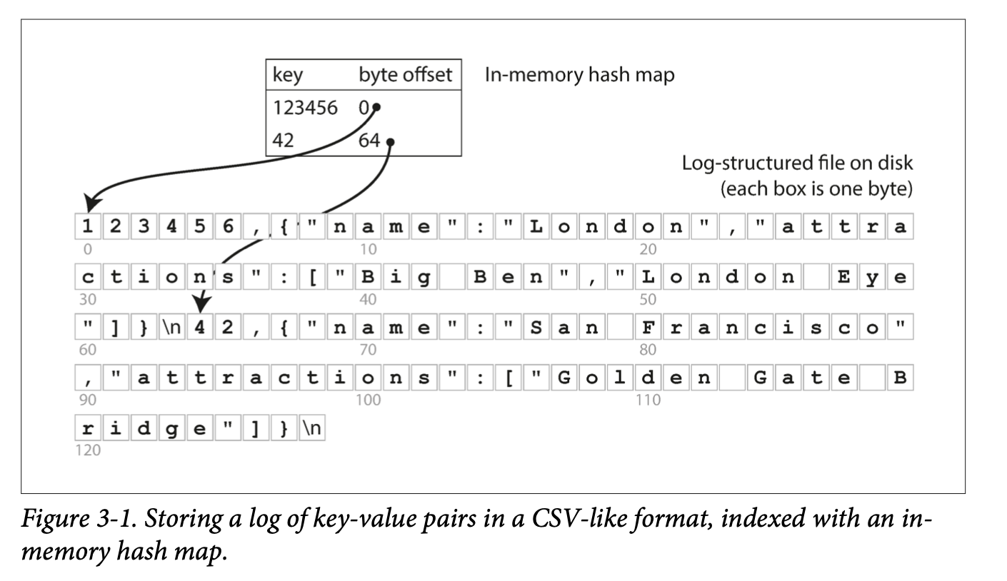
• Hash Indexes are for key-value data and are similar to a dictionary, which is usually implemented as a hash map (hash table).
• If the database writes only append new entires to a file, the hash table can simply store key to byte offset in the data file. The hash table (with keys) has to fit into memory for quick look up performance, but the values don’t have to fit into memory.
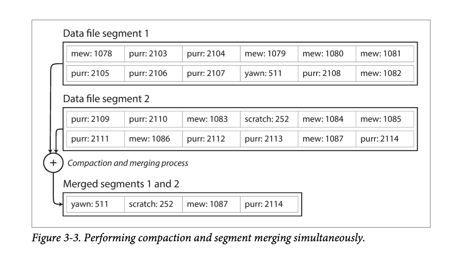
• To avoid the disk run out of space, a good solution is to break logs into segments and perform compaction (remove duplicate keys). Further, file segments can be merged while performing compaction. We can use a background thread to perform merging and compaction and switch our read request to the newly created segment when they are read. Afterwards, old segments can be deleted.
• Bitcask (the default storage engine in Riak) does it like that. The only requirement it has is that all the keys fit in the available RAM. Values can use more space than there is available in memory, since they can be loaded from disk.
• A storage engine like Bitcask is well suited to situations where the value for each key is updated frequently. There are a lot of writes, but there are too many distinct keys, you have a large number of writes per key, but it's feasible to keep all keys in memory.
• There are a few details for a real implementation of the idea above
  • Use bytes instead of CSV
  • Deletes are adding a special log entry to the data file (tombstone) and the data will be removed during merging and compaction.
  • Index will need to be snapshotted for fast crash recovery (compared to re-indexing).
  • Checksums are required for detecting partially written records.
  • Writes has to strictly be in sequential order. Many implementation choose to have one writer thread.
• Why append-only logs are good
  • Sequential writes are much faster than random writes, especially on magnetic spinning-disk hard drives and to some extent SSDs.
  • Concurrency and crash recovery are much simpler if segment files are append-only or immutable.
  • Merging old segments avoids data fragmentation.
• What are the limitations of hash table indexes?
  • Hash table must fit into memory. If there are too many keys, it will not fit.
  • Range queries are not efficient.

• The Sorted String Table (SSTable) requires each segment file to be sorted by key. It has the following advantages.
  • Merging segments is simple and efficient.
  • We no longer require offset of every single key for efficient lookup. One key for every few kilobytes of segment file is usually sufficient.
  • Since reading requires a linear scan in between indexed keys, we can group those records and compress them to save storage or I/O bandwidth.

• While maintaining a sorted structure on disk is possible (B-Trees), red-black trees or AVL trees can be used to keep logs sorted in memory. The flow is as follows:
  • When a write comes in, insert the entry to the in-memory data structure (sometimes called memtable).
  • When memtable gets bigger than some threshold (a few megabytes), create a new memtable to handle new writes, and write the old memtable to disk.
  • For reads, first try to find the key in memtable, and in the latest segment, and in the second last segment.
  • Occasionally, run a merging and compaction process to combine segment files.
• The issue with this scheme is that in-memory data will be lost if the database crashes. We can keep a separate unsorted log for recovery and this log can be discarded whenever a memtable is dumped to disk.
• This indexing structure is named Log-Structure Merge-Tree (LSM-Tree).

• The algorithm here is used by LevelDB and RocksDB, which are key-value storage libraries to be used in other applications. Similar storage systems are also used in Cassandra and HBase.
• Systems that uses the principle of merging and compacting sorted files are often called LSM systems.

• A look up can take a long time if the entry does not exist in any of the memtable. Bloom filters can be used to solve this issue.
• There are two major strategies to determine the order and timing of merging and compaction: size-tiered (HBase, Cassandra) and level compaction (LevelDB, RockDB, Cassandra).
  • Size-tiered: newer and smaller SSTables are merged into larger ones.
  • Level: The key range is split up into several SSTables and older data is moved to separate “levels,” which allows compaction to proceed more incrementally and use less disk space.
• LSM-tree: Write throughput is high. Can efficiently index data much larger than memory.

• While log-structured indexes are gaining acceptance, B-tree is the most widely used indexing structure.
• B-trees is the standard index implementation for almost all relational databases and most non-relational databases.
• B-trees also keep key-value entires sorted by key, which allows quick value lookups and range queries.
• Log-structure indexes breaks databases down into variable length segments (several mbs or more), while B-tree breaks databases down into a fixed-size blocks or pages (4KB traditionally, but depends on underlying hardware).
• Each page can be identified by an address or location, which can be stored in another page on disk.
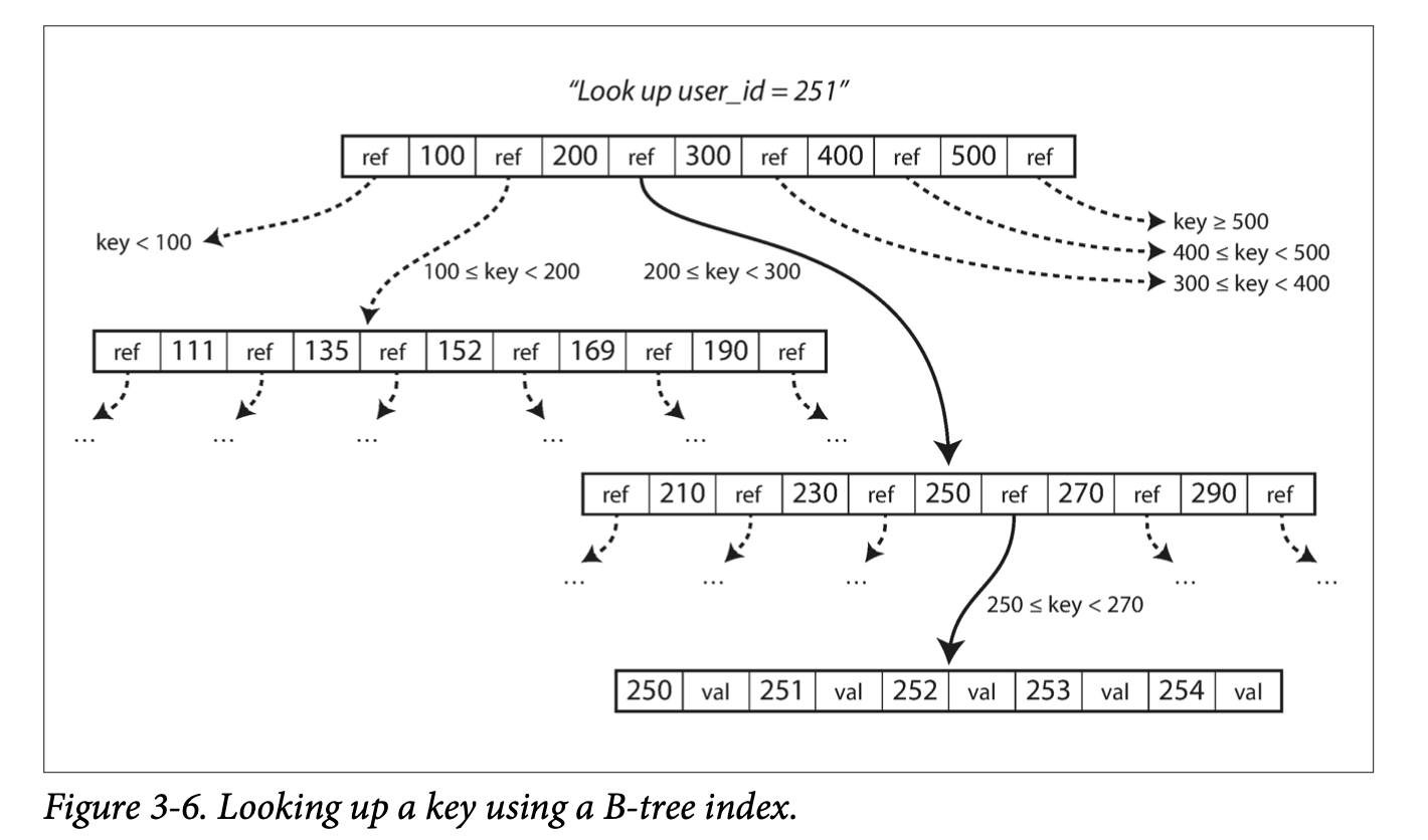
• A root page contains the full range of keys (or reference to pages containing the full range) and is where query start.
• A leaf page contains only individual keys, which contains the value inline or reference to where the values can be found.
• The branching factor is the number of references to a child page in one page of a B-tree.
• When changing values in B-trees, the page containing the value is looked up, modified, and written back to disk.
• When adding new values, first, the page whose range contains the key is looked up. If there is extra space in the page, the key-value entry is simply added, else, the page is split into two halves and the parent page is updated to account for the new file structure.
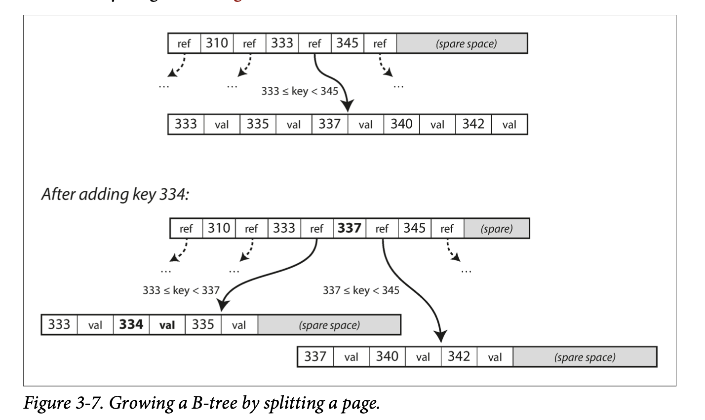
• The algorithm above ensures a B-tree with n nodes is always balanced and has a depth of O(logn).

• When changing values or splitting pages, the B-tree overwrites data on disk. This is a risky operation. If anything crashes during an overwrite, the index could be corrupted.
• To make B-tree more resilient to such failures, a common solution is to include an write-ahead-log (WAL, or redo log), which every B-tree modification is first written to. In case of failure, this log can be used to restore the B-tree back to a consistent state.
• Care should also be taken when multiple threads may access the B-tree at the same time. An inconsistent state could be read during an update. Latches (lightweight locks) can be placed to protect the tree’s integrity.

• Just to mention a few optimizations:
  • Copy-on-write and atomic to remove the need to maintain a WAL for crashes
  • Key compression by storing essential information for acting as boundaries.
  • Arrange page on disk such that pages appear in sequential order on disk.
  • Additional pointers (such as left, right siblings) to allow efficient scanning of keys in order without jumping back to parents.
  • Fractal trees to reduce disk seeks.

• Typically, B-Trees are faster for reads and LSM-Trees are faster for writes. The actual performance for a specific system would require benchmarking.

• Both B-Tree and LSM-tree indexes would require writing a piece of data to disk multiple times on write. This effect is known as write amplification. In write heavy applications, write amplification would directly impact performance.
• LSM-trees are typically able to sustain higher write throughput due to two main reasons: a lower write amplification and a sequential write (especially on magnetic hard drives).
• LSM-trees can be compressed better and have lower fragmentation due to rewriting of SSTables.
• Even on SSDs, LSM-trees are still advantages as it represents data more compactly and allows more read and write requests within the same bandwidth.

• The compaction process of LSM-trees can sometimes interfere with reads and writes, as reads and writes can be blocked by the compaction process on disk resources. Although the impact on average response time is usually small, this could greatly increase high-percentage response time.
• If write throughput is high and compaction is not configured correctly, it is not impossible that compaction can’t keep up with incoming writes. Unmerged segments will then grow until disk space is all used. This effect has to be actively monitored.
• Since each key only appears once in a B-tree, B-trees are more attractive in databases when transaction isolation is implemented using locks on range of keys.

• Secondary indexes can be created from a key-value index. The main difference between primary and secondary indexes is that secondary indexes are not unique. This can be solved two ways:
  • Make the value in the index a list of matching row identifiers.
  • Make each key unique by adding a row identifier to the secondary key.
• Both B-trees and log-structured indexes can be used as secondary indexes.

• In a key-value pair, the key is used to locate the entry and the value can be either the actual data or a reference to the storage location (known as a heap file). Using heap files is common for building multiple secondary indexes to reduce duplication.
• When updating values without changing keys, if the new value is no larger than old data, the value can be directly overwritten, and if the new value is larger, either all indexes needs to be updated or a forwarding pointer can be left in the old record.
• Sometimes, the extra hop to the heap file is too expensive for reads, and the indexed row is stored directly in the index. This is called a clustered index.
• A compromise between a non-clustered index and a clustered index is a covering index or index with included columns, where only some columns are stored within the index.

• Multi-column indexes are created for querying rows using multiple columns of a table.
• The concatenate index is the most common multi-column index. This is done by simply concatenating fields together into one key. However the index is useless when a query is based on only one column.
• To index a two-dimensional location database (with latitude and longitude), we can use a space-filling curve and use a regular B-tree index. Specialized spatial index such as R-trees are also used.

• Some applications require searching for a similar key. This can be done by fuzzy indexes.
• For example, Lucene allows searching for words within edit distance 1. In Lucene, the in-memory index is a finite state automaton over the characters in the keys (similar to a trie). This automaton can then be transformed into a Levenshtein automaton, which supports efficient search for words within a given distance.

• Some in-memory key-value stores, such as Memcached, are intended for caching only, where data is lost when the machine restarts. Some other in-memory databases aim for durability, which can be achieved with special hardware and saving change logs and snapshots to disk.
• Counterintuitively, in-memory databases are faster mainly because they avoid serialization and deserialization between in-memory structures and binaries, not because of the disk read and write time.
• In-memory databases could also provide data models that are hard to implement with disk-based indexes, such as priority queues, stacks.
• The anti-caching approach, where the least-recently-used data is dumped to disk when there is not enough memory and loaded back when queried, enables in-memory databases to support larger-than-memory databases. Yet the index would still have to fit into memory.

• The term transaction (an entry) was coined in the early days of databases, where commercial transactions were the main entries in databases. Although the data in databases are now different, the access pattern: looking up a few entries by key, inserting or updating data based on user input, remains the same and is referred to as online transaction processing (OLTP).
• Databases nowadays are also used for data analytics. The access pattern: scanning through the whole database and performing aggregation, is a very different from OLTP. This pattern is referred to as the online analytic processing (OLAP).

• Starting 1980s, people stopped using OLTP systems for OLAP applications. The data for analytics is hosted in a separate database - a data warehouse.

• OLTP is expected to be highly available with low latency, so it is not ideal to run analytics on OLTP databases.
• A data warehouse contains a read-only copy of the data in OLTP systems through periodic dumps or stream of updates.
• The process of getting data from OLTP systems to data warehouses is called Extract-Transform-Load (ETL).

• Data warehouses, separate from OLTP systems, can be optimized for analytics access patterns.
• The indexing algorithms mentioned above are for OLTP systems, not analytics.

• Although most data warehouses use a relational data model, the internals of the systems is very different as they are optimized for different access patterns.
• Although some products combines OLTP with data warehousing (Microsoft SQL, SAP HANA), they are increasingly becoming two separate systems.

• Many data warehousing systems uses a star-schema, whose center is a fact table, where each row represents an event. The fact table uses foreign keys to refer to other tables (called dimension tables) for entities (with extra information) that was involved in the event.
• The snowflake schema further breaks dimensions down into sub-dimensions. Snowflake schemas are more normalized than star schemas, but star schemas are easier for analysts to work with.
• A typical data warehouse, tables could be very wide (up to several hundred columns), and dimension tables could also be very wide.

• A typical data warehouse query only access several rows.
• In most OLTP and document databases, storage is laid out in a row-oriented fashion, meaning all data from one row are stored next to each other. This is inefficient for queries which only accesses a few columns of all rows. The whole row will have to be read and filtered down to the columns of interest.
• In column-oriented storage, data of all rows from each column are stored together. It relies on each file containing the rows in the same order.

• Column-oriented storage often lends itself to good compression.
• Bitmap encoding of distinct values in a column can lead to good compression. Further, if the bitmap is sparse, we can use run-length encoding for more compression.
• Bitmap indexes are good for “equal” and “contain” queries.

• Although storing column in insertion order is easy, we can choose to sort them based on what queries are common.
• The administrator can specify a column for the database to be sorted in as well as a second column to break ties.
• The sorted columns would be much easier to compress if there are not a lot of distinct values in the column.

• Since data warehouse usually store multiple copies of the same data, it could use a different sort order for each replication, so that we can use different datasets for different queries.
• An analogy of multiple sorted orders to row-based databases is multiple secondary indexes. The difference is that row-based databases stores the data in one place and use pointers in secondary indexes, while column stores don’t use any pointers.

• Sorted columns optimizes for read-only queries, yet writes are more difficult.
• In-place updates would require rewriting the whole column on every write. Instead, we can use a LSM-tree like structure where a in-memory store buffers the new writes. When enough new writes are accumulated, they are then merged with the column files and written to new files in bulk.
• Queries, in this case, would require reading data from both disk and the in-memory store. This will be hidden within the engine and invisible to the user.

• Since many queries involves aggregation functions, a data warehouse can cache materialized aggregates to avoid recomputing expensive queries.
• One way of creating such a cache is a materialized view, which is defined like a standard view, but with results stored on disk, while virtual views are expanded and processed at query time.
• Updating materialized view, when data changes, is expensive, and therefore materialized views are not used in OLTP systems often.
• A common special case of materialized view is a data cube or OLAP cube, where data is pre-summarized over each dimension. This enables fast queries with precomputed queries, yet a data cube may not have the flexibility as raw data.

• Evolvability is important for maintainability in the long term, as applications inevitably change over time.
• Relational databases ensures all data conforms to the same format. The schema can be changed, but there is always only one schema.
• Schema-on-read databases can contain data a mix of data with older and newer formats.
• For larger applications, schema updates often cannot happen at the same time:
  • Server side application can perform rolling-upgrade: a few nodes are updated at a time. No service downtime required.
  • Client side application depends entirely on the user.
• This means old and new versions of the code and data may exist at the same time.
• We define backward compatibility as: newer code can read data written by older code. This is usually easier.
• We define forward compatibility as: older code can read data written by newer code. This could be tricker.

• Data usually are in one the following two representation:
  • In memory, data is kept in objects, structs, list, arrays, hash tables, trees, etc. Those data structures are optimized for efficient access and manipulation.
  • When data is written to a file or sent over the network, data are encoded into a sequence of bytes.
• Translating from in-memory representation to a byte sequence is called encoding, serialization, or marshalling. The revers is called decoding, parsing, deserialization, unmarshalling. This book uses the terms encoding and decoding.

• Java has Serializable, Ruby has Marshal, python has pikle and so on. Although language-specific formats comes with built-in support and are convenient, they have a few issues.
  • Encoding is tied to a specific programming language, and cross-language reads are difficult. Migration to another language could be very expensive.
  • Decoding needs to be able to instantiating arbitrary classes, which could be a security problem.
  • Versioning is often an afterthought, and forward and backward compatibility is generally overlooked.
  • Efficiency is often an afterthought. Java's serialization is notorious for bad performance and bloated encoding.
• TLDR. Don’t use them.

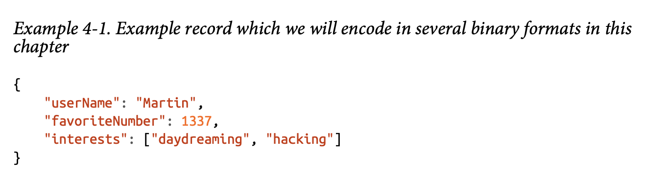
• JSON, XML, CSV are textual formats and somewhat human readable, yet they have the following problems:
  • There is a lot of ambiguity around encoding of numbers. In XML and CSV, a numeric string and a number are the same. JSON doesn’t distinguish integers and floating-point numbers. Also, integers greater than 2^53 cannot be exactly represented by a IEEE 754 double-precision floating-point number.
  • JSON and XML support Unicode character strings well but they don’t support binary strings.
  • While there is schema support for XML and JSON, many JSON-based tools don’t use schemas. Applications that don’t use schemas need to hardcode the encoding and decoding logic.
  • CSV does not have a schema, so encoding and decoding logic will have to be hardcoded. Also, not all CSV parsers handles escaping rules correctly.
• Despite the flaws, XML, JSON, and CSV are good enough for many purposes as long as application developers agree on the format.

• For bigdata, the efficiency of encoding can have a larger impact.
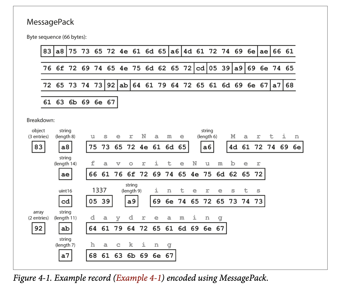
• Binary formats for JSON and XML have been developed but only adopted in niches.
• Those binary representation usually keep the data model unchanged and keeps field names within the encoded data.
• The book gave a MessagePack example where the data was compressed from 81 bytes to 61 bytes.

• Thrift and Protocol Buffers (protobuf) require a schema for encoding and decoding. They have their own schema definition language, which can then be use to generate code for multiple languages.
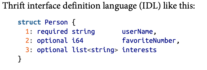
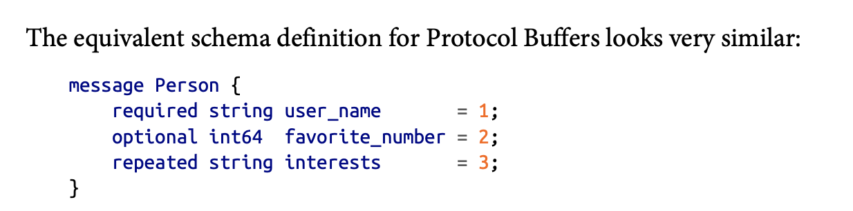
• Since Thrift and Protocol Buffers encodes the schema in code, the encoding does not need the field names but only field tags (positive integers).
• Thrift has two binary encoding formats: BinaryProtocol and CompactProtocol. CompactProtocol packs field type and tag number into a single byte and uses variable length encoding for integers.
• Thrift and Protocol Buffers allow a field to be optional, yet the actual binary encoding does not have this information. The difference is only at run-time, where read a missing required field would result in an exception.

• Each field in Thrift and Protocol Buffers has a tag number and a data type. Since each field is identified only by the field tag, the name can be changed and the field tag number cannot be changed.
• For forward compatiblility, old code can simply skip the fields with unknown tags. For backward compatibility, as long as the newly added field is optional, new code can read data without the new optional field without throwing exceptions.

• Changing datatypes is trickier. Changing a 64-bit integer to 32-bit integer would lose precision or get truncated.
• Protocol Buffers does not have a list or array datatype, but has a repeated marker for fields that can appear multiple times. It is okay to change an optional field into a repeated field. New code sees a list of zero or one elements; old code reading new data sees the last element in the list. Thrift does not have this flexibility.

• Arvo has two schema languages, one Arvo IDL for human editing and one JSON based that is more machine-readable.
• There are no tag numbers in the schema. The encoding is a concatenation of field values.

• Arvo supports schema evolvability by keeping track of the writer’s schema and compare it with the reader’s schema.
• The reader’s and writer’s schema don’t have to be the same but only have to be compatible.

• To maintain compatibility, one can only add or remove a field with a default value.
• Note that Arvo does not allow nulls to be a default value unless a union type, which includes a null, is the type of the field. As a result, Arvo does not have optional and required.
• Changing the datatype is possible as long as Arvo can convert the type. Changing the name of the field is done by adding aliases of field names, so a new reader’s schema can match old writer’s schema. Note this is only backward compatible, not forward compatible.

• Since it is inefficient to encode the writer’s schema with each data entry, how the writer’s schema is handled depends on the context.
  • Storing many entries of the same schema: the writer’s schema can be written once at the beginning of the file.
  • Database with individually written records: one can include a version number for each record and store a map of schema version to schema in a separate database.
  • Sending data over a network: The schema can be negotiated during the connection setup time if the communication is bidirectional.
• A database of schema versions is a useful thing that can also be used as a documentation of the evolution history.

• Since Arvo does not use tags for fields, it is friendlier to dynamic generated schemas. No code generation is required when the schema changes. For example, if we have an application that dumps relational database contents to disk, we do not need to perform code generation a new schema every time the database adds a new field.

• Code generation is more aligned with statically typed languages as it allows efficient in-memory structures to be used for decoded data, and it allows type checking and autocompletion in IDEs. However, for dynamically typed languages code generation becomes a burden, as they usually avoid an explicit compilation step.
• Arvo provides optional code generation for statically typed languages, but it can be used without any code generation as long as you have the writer’s schema. This is especially useful for working with dynamically typed data processing languages.

• Compared to JSON, XML, and CSV, formats with a schema, such as Protocol Buffer, Thrift, and Arvo have the following good properties:
  • They are simpler to implement.
  • They are much more compact.
  • The schema is a form of documentation.
  • Keeping a database of schemas allows one to check forward and backward compatibility before anything is deployed.
  • Automatic code generation for statically typed languages.

• The most common ways of how data flows between applications are:
  • through database,
  • through service calls,
  • and through asynchronous message passing.

• Data can be sent from one application to a different application or the application’s future self through databases.
• A process that writes to a database encodes the data, and a process that reads data from a database decodes the data.
• Both backward and forward compatibility are required here.
• An old process reading and writing a record of new data will need to preserve the unknown fields.

• Databases may persist data for years, and it is common that data outlives code.
• Rewriting (migrating) is expensive, most relational databases allow simple schema changes, such as adding a new column with a null default value without rewriting existing data. When an old row is read, the database fills in nulls for any columns that are missing.
• Schema evolution allows the entire database to appear as if it was encoded with a single schema, even if the binary format was encoded with different versions of the schema.
• Avro has sophisticated schema evolution rules that can allow a database to appear as if was encoded with a single schema, even though the underlying storage may contain records encoded with previous schema versions.

• When taking a snapshot or dumping data into a data warehouse, one can encode all data in the latest schema.

• Data can be sent from a one application (client) to another application (server) through network over the API (service) the server exposes.
• HTTP is the transport protocol and is independent of the server-client agreement of the API.
• A few examples of clients:
  • Web browsers retrieves data using HTTP GET requests and submits data through HTTP POST requests.
  • A native application could also make requests to a server and a client-side JavaScript application can use XMLHttpRequest to become an HTTP client (Ajax). In this case the response is usually not human readable but for further processing by the client.
  • A server can be a client of another service. Breaking down a monolithic service into smaller services is referred to as the microservices architecture or service-oriented architecture.
• The goal for microservices architecture is to make each subservice independently deployable and evolvable. Therefore, we will need both forward and backward compatibility for the binary encodings of data.

• When HTTP is used as the protocol for talking to the service, it is called a web service, for example:
  • A client application making requests to a service over HTTP over public internet.
  • A service making requests to services within the same organization. Software that supports such services is sometimes called middleware.)
  • A service making requests to services owned by a different organization.
• There are two approaches for designing the API for web services REST and SOAP.
• REST uses simple data formats, URLs for identifying resources, and HTTP features for cache control, authentication and content type negotiation. APIs designed based on REST principles are called RESTful.
• SOAP is a XML-based protocol. While it uses HTTP, it avoids using HTTP features. SOAP APIs are described using Web Services Description Language (WSDL), which enables code generation. WSDL is complicated and requires tool support for constructing requests manually.
• REST has been gaining popularity.

• The RPC model treats a request to a remote network service the same as a calling a function within the same process (this is called location transparency.) This approach has the following issues:
  • A network request is more unpredictable than a local function call.
  • A local function call returns a result, throws an exception, or never returns, but a network call may return without a result, due to a timeout.
  • Retrying a failed network request is not the right solution, as the request could have gone through, but the response was lost.
  • The run time for the function is unpredictable.
  • Passing references to objects in local memory requires encoding the whole object and could be expensive for large objects.
  • The client and server may be implemented in different languages, so the framework must handle the datatype translations.

• The new generation of RPC frameworks is more explicit about the fact that a remote call is different from a local call, e.g., Finagle and Rest.li use futures (promises) to encapsulate asynchronous actions that may fail. Some of those frameworks provide service discovery to allow clients to find out which IP address and port number it can find a particular service.
• Custom RPC protocols with binary encoding can achieve better performance than JSON over REST, but RESTful APIs are easier to test and is supported by all mainstream programming languages.

• We can assume the server will always be updated before the clients, so we only need backward compatibility on requests and forward compatibility on responses.
• The compatibilities of a RPC scheme are directly inherited by the binary encoding scheme it uses.
• RESTful APIs usually uses JSON for responses or URI-encoded/form-encoded for requests. Therefore, adding optional new request parameters or response fields maintains compatible.
• For public APIs, the provider has no control over its clients and will have to maintain them for a long time.
• There is no agreement on how API versioning should work. For RESTful APIs, common approaches are to use a version number in the URL or in the HTTP Accept header.

• Asynchronous message-passing systems are somewhere between RPC and databases. Data is sent from a process to another process with low latency through a message broker, which stores the message temporarily.
• Using a message broker, compare to direct RPC, the advantages are:
  • It can act as a buffer to improve reliability.
  • It can redeliver messages to a process that has crashed.
  • The sender does not need to know the IP or port of the recipient.
  • It allows one message to be sent to multiple receivers.
  • It decouples the sender and receiver.
• The communication is one-way and asynchronous. The sender doesn’t wait for the response from the receiver.

• Message brokers are used as follows. The producer sends a message to a named queue or topic, and the broker ensures the message is delivered to the consumers or subscribers of that queue or topic. There could be many producers and consumers on the same topic.
• Ideally the messages should be encoded by a forward and backward compatible scheme. If a consumer republishes a message to another topic, it may need to preserve unknown fields.

• The actor model is a programming model for concurrency in a single process. Each actor may have its own state and communicates with other actors through sending and receiving asynchronous messages.
• In distributed actor frameworks, the actor model is used to scale an application across multiple nodes. The same message-passing mechanism is used.
• Location transparency works better in the actor model than RPC, since the model already assumes the messages could be lost.
• Three popular distributed actor frameworks: Akka, Orleans, Erlang OPT.

• Reasons for replication:
  • Store data closer to users to reduce latency.
  • Improve availability.
  • Scale throughput
• The challenge is not storing the data, but handling changes to replicated data.
• There are three popular algorithms: single-leader, multi-leader, and leaderless replication.

Every node that keeps a copy of data is a replica. Obvious question is: how do we make sure that the data on all the replicas is the same? The most common approach for this is leader-based replication. In this approach:

1. Only the leader accepts writes.
2. The followers read off a replication log and apply all the writes in the same order that they were processed by the leader.
3. A client can query either the leader or any of its followers for read requests.

So here, the followers are read-only, while writes are only accepted by the leader. This approach is used by MySQL, PostgreSQL etc., as well as non-relational databases like MongoDB, RethinkDB, and Espresso.

With Synchronous replication, the leader must wait for a positive acknowledgement that the data has been replicated from at least one of the followers before terming the write as successful, while with Asynchronous replication, the leader does not have to wait.

The advantage of synchronous replication is that if the leader suddenly fails, we are guaranteed that the data is available on the follower.

The disadvantage is that if the synchronous follower does not respond (say it has crashed or there's a network delay or something else), the write cannot be processed. A leader must block all writes and wait until the synchronous replica is available again. Therefore, it's impractical for all the followers to be synchronous, since just one node failure can cause the system to become unavailable.

In practice, enabling synchronous replication on a database usually means that one of the followers is synchronous, and the others are asynchronous. If the synchronous one is down, one of the asynchronous followers is made synchronous. This configuration is sometimes called semi-synchronous.

In this approach, if the leaders fails and is not recoverable, any writes that have not been replicated to followers are lost. An advantage of this approach though, is that the leader can continue processing writes, even if all its followers have fallen behind.

There's some research into how to prevent asynchronous-performance like systems from losing data if the leader fails. A new replication method called Chain replication is a variant of synchronous replication that aims to provide good performance and availability without losing data.

New followers can be added to an existing cluster to replace a failed node, or to add an additional replica. The next question is how to ensure the new follower has an accurate copy of the leader's data?

1. Take a consistent snapshot of the leader's db at some point in time. It's possible to do this without taking a lock on the entire db. Most databases have this feature.
2. Copy the snapshot to the follower node.
3. The follower then requests all the data changes that happened since the snapshot was taken.
4. When the follower has processed the log of changes since the snapshot, we say it has caught up. In some systems, this process is fully automated, while in others, it is manually performed by an administrator.

Any node can fail, therefore, we need to keep the system running despite individual node failures, and minimize the impact of a node outage. How do we achieve high availability with leader-based replication?

Each follower typically keeps a local log of the data changes it has received from the leader. If a follower node fails, it can compare its local log to the replication log maintained by the leader, and then process all the data changes that occurred when the follower was disconnected.

This is trickier: One of the nodes needs to be promoted to be the new leader, clients need to be reconfigured to send their writes to the new leader, and the other followers need to start consuming data changes from the new leader. This whole process is called a failover. Failover can be handled manually or automatically.

An automatic failover consists of:

1. Determining that the leader has failed: Many things could go wrong: crashes, power outages, network issues etc. There's no foolproof way of determining what has gone wrong, so most systems use a timeout. If the leader does not respond within a given interval, it's assumed to be dead.
2. Choosing a new leader: This can be done through an election process (where the new leader is chosen by a majority of the remaining replicas), or a new leader could be appointed by a previously elected controller node. The best candidate for leadership is typically the one with the most up-to-date data changes from the old leader (to minimize data loss)
3. Reconfiguring the system to use the new leader: Clients need to send write requests to the new leader, and followers need to process the replication log from the new leader. The system also needs to ensure that when the old leader comes back, it does not believe that it is still the leader. It must become a follower.

There are a number of things that can go wrong during the failover process:

• For asynchronous systems, we may have to discard some writes if they have not been processed on a follower at the time of the leader failure. This violates clients' durability expectations.
• Discarding writes is especially dangerous if other storage systems are coordinated with the database contents. For example, say an autoincrementing counter is used as a MySQL primary key and a redis store key, if the old leader fails and some writes have not been processed, the new leader could begin using some primary keys which have already been assigned in redis. This will lead to inconsistencies in the data, and it's what happened to Github (https://github.blog/2012-09-14-github-availability-this-week/).
• In fault scenarios, we could have two nodes both believe that they are the leader: split brain. Data is likely to be lost/corrupted if both leaders accept writes and there's no process for resolving conflicts. Some systems have a mechanism to shut down one node if two leaders are detected. This mechanism needs to be designed properly though, or what happened at Github can happen again( https://github.blog/2012-12-26-downtime-last-saturday/)
• It's difficult to determine the right timeout before the leader is declared dead. If it's too long, it means a longer time to recovery in the case where the leader fails. If it's too short, we can have unnecessary failovers, since a temporary load spike could cause a node's response time to increase above the timeout, or a network glitch could cause delayed packets. If the system is already struggling with high load or network problems, unnecessary failover can make the situation worse.

Several replication methods are used in leader-based replication. These include:

In this approach, the leader logs every write request (statement) that it executes, and sends the statement log to every follower. Each follower parses and executes the SQL statement as if it had been received from a client.

A problem with this approach is that a statement can have different effects on different followers. A statement that calls a nondeterministic function such as NOW() or RAND() will likely have a different value on each replica. If statements use an autoincrementing column, they must be executed in exactly the same order on each replica, or else they may have a different effect. This can be limiting when executing multiple concurrent transactions, as statements without any causal dependencies can be executed in any order. Statements with side effects (e.g. triggers, stored procedures) may result in different side effects occurring on each replica, unless the side effects are deterministic. Some databases work around this issues by requiring transactions to be deterministic, or configuring the leader to replace nondeterministic function calls with a fixed return value.

The log is an append-only sequence of bytes containing all writes to the db. Besides writing the log to disk, the leader can also send the log to its followers across the network.

The main disadvantage of this approach is that the log describes the data on a low level. It details which bytes were changed in which disk blocks. This makes the replication closely coupled to the storage engine. Meaning that if the storage engine changes in another version, we cannot have different versions running on the leader and the followers, which prevents us from making zero-downtime upgrades.

This logs the changes that have occurred at the granularity of a row. Meaning that:

• For an inserted row, the log contains the new values of all columns.
• For a deleted row , the log contains enough information to identify the deleted row. Typically the primary key, but it could also log the old values of all columns.
• For an updated row, it contains enough information to identify the updated row, and the new values of all columns.

This decouples the logical log from the storage engine internals. Thus, it makes it easier for external applications (say a data warehouse for offline analysis, or for building custom indexes and caches) to parse. This technique is called change data capture.

This involves handling replication within the application code. It provides flexibility in dealing with things like: replicating only a subset of data, conflict resolution logic, replicating from one kind of database to another etc. Trigger and Stored procedures provide this functionality. This method has more overhead than other replication methods, and is more prone to bugs and limitations than the database's built-in replication.

Eventual Consistency: If an application reads from an asynchronous follower, it may see outdated information if the follower has fallen the leader. This inconsistency is a temporary state, and the followers will eventually catchup. That's eventual consistency.

The delay between when a write happens on a leader and gets reflected on a follower is replication lag.

Other Consistency Levels There are a number of issues that can occur as a result of replication lag. In this section, I'll summarize them under the minimum consistency level needed to prevent it from happening.

Read-after-write consistency, also known as read-your-writes consistency is a guarantee that if the user reloads the page, they will always see any updates they submitted themselves.

How to implement it:

• When reading something that the user may have modified, read it from the leader. For example, user profile information on a social network is normally only editable by the owner. A simple rule is always read the user's own profile from the leader.
• You could track the time of the latest update and, for one minute after the last update, make all reads from the leader.
• The client can remember the timestamp of the most recent write, then the system can ensure that the replica serving any reads for that user reflects updates at least until that timestamp.
• If your replicas are distributed across multiple datacenters, then any request needs to be routed to the datacenter that contains the leader. Another complication is that the same user is accessing your service from multiple devices, you may want to provide cross-device read-after-write consistency.

Some additional issues to consider:

• Remembering the timestamp of the user's last update becomes more difficult. The metadata will need to be centralised.
• If replicas are distributed across datacenters, there is no guarantee that connections from different devices will be routed to the same datacenter. You may need to route requests from all of a user's devices to the same datacenter.

Because of followers falling behind, it's possible for a user to see things moving backward in time.

When you read data, you may see an old value; monotonic reads only means that if one user makes several reads in sequence, they will not see time go backward.

Make sure that each user always makes their reads from the same replica. The replica can be chosen based on a hash of the user ID. If the replica fails, the user's queries will need to be rerouted to another replica.

Another anomaly that can occur as a result of replication lag is a violation of causality. Meaning that a sequence of writes that occur in one order might be read in another order. This can especially happen in distributed databases where different partitions operate independently and there's no global ordering of writes. Consistent prefix reads is a guarantee that prevents this kind of problem.

One solution is to ensure that causally related writes are always written to the same partition, but this cannot always be done efficiently.

Application developers should ideally not have to worry about subtle replication issues and should trust that their databases "do the right thing". This is why transactions exist. They allow databases to provide stronger guarantees about things like consistency. However, many distributed databases have abandoned transactions because of the complexity, and have asserted that eventual consistency is inevitable. Martin discusses these claims later in the chapter.

The downside of single-leader replication is that all writes must go through that leader. If the leader is down, or a connection can't be made for whatever reason, you can't write to the database.

Multi-leader/Master-master/Active-Active replication allows more than one node to accept writes. Each leader accepts writes from a client, and acts as a follower by accepting the writes on other leaders.

Here, each datacenter can have its own leader. This has a better performance for writes, since every write can be processed in its local datacenter (as opposed to being transmitted to a remote datacenter) and replicated asynchronously to other datacenters. It also means that if a datacenter is down, each data center can continue operating independently of the others.

Multi-leader replication has the disadvantage that the same data may be concurrently modified in two different datacenters, and so there needs to be a way to handle conflicts.

Some applications need to work even when offline. Say mobile apps for example, apps like Google Calendar need to accept writes even when the user is not connected to the internet. These writes are then asynchronously replicated to other nodes when the user is connected again. In this setup, each device stores data in its local database. Meaning that each device essentially acts like a leader. CouchDB is designed for this mode of operation apparently.

Real-time collaborative editing applications like Confluence and Google Docs allow several people edit a document at the same time. This is also a database replication problem. Each user that edits a document has their changes saved to a local replica (webbrowser cache), from which it is then replicated asynchronously.

For faster collaboration, the unit of change can be a single keystroke. That is, after a keystroke is saved, it should be replicated.

Multi-leader replication has the big disadvantage that write conflicts can occur, which requires conflict resolution.

If two users change the same record, the writes may be successfully applied to their local leader. However, when the writes are asynchronously replicated, a conflict will be detected. This does not happen in a single-leader database.

In theory, we could make conflict detection synchronous, meaning that we wait for the write to be replicated to all replicas before telling the user that the write was successful. Doing this will make one lose the main advantage of multi-leader replication though, which is allowing each replica to accept writes independently. Use single-leader replication if you want synchronous conflict detection.

Conflict avoidance is the simplest strategy for dealing with conflicts. Conflicts can be avoided by ensuring that all the writes for a particular record go through the same leader. For example, you can make all the writes for a user go to the same datacenter, and use the leader there for reading and writing. This of course has a downside that if a datacenter fails, traffic needs to be rerouted to another datacenter, and there's a possibility of concurrent writes on different leaders, which could break down conflict avoidance.

On single-leader, the last write determines the final value of the field. In multi-leader, it's not clear what the final value should be.

The database must resolve the conflict in a convergent way, all replicas must arrive a the same final value when all changes have been replicated. Different ways of achieving convergent conflict resolution.

• Giving each write a unique ID ( e.g. a timestamp, UUID etc.), pick the write with the highest ID as the winner, and throw away the other writes. If timestamp is used, that's Last write wins, it's popular, but also prone to data loss.
• Giving each replica a unique ID, and letting writes from the higher-number replica always take precedence over writes from a lower-number replica. This is also prone to data loss.
• Recording the conflict in an explicit data structure that preserves the information, and writing application code that resolves the conflict at some later time (e.g. by prompting the user).
• Merge the values together e.g. ordering them alphabetically.

The most appropriate conflict resolution method may depend on the application, and thus, multi-leader replication tools often let users write conflict resolution logic using application code. The code may be executed on read or on write:

On write: When the database detects a conflict in the log of replicated changes, it calls the conflict handler. The handler typically runs in a background process and must execute quickly. It has no user interaction. On Read: Conflicting writes are stored. However, when the data is read, the multiple versions of the data are returned to the user, either for the user to resolve them or for automatic resolution. Automatic conflict resolution is a difficult problem, but there are some research ideas being used today:

• Conflict-free replicated datatypes (CRDTs) - Used in Riak 2.0
• Mergeable persistent data structure - Similar to Git. Tracks history explicitly
• Operational transformation: Algorithm behind Google Docs. It's still an open area of research though.

A replication topology is the path through which writes are propagated from one node to another. The most general topology is all-to-all, where each leader sends its writes to every other leader. Other types are circular topology and star topology.

All-to-all topology is more fault tolerant than the circular and star topologies because in those topologies, one node failing can interrupt the flow of replication messages across other nodes, making them unable to communicate until the node is fixed.

In this replication style, the concept of a leader is abandoned, and any replica can typically accept writes from clients directly.

This style is used by Amazon for its in-house Dynamo system. Riak, Cassandra and Voldermort also use this model. These are called Dynamo style systems.

In some leaderless implementations, the client writes directly to several replicas, while in others there's a coordinator node that does this on behalf of the client. Unlike a leader database though, this coordinator does not enforce any ordering of the writes.

Say there are 3 replicas and one of the replicas goes down. A client could write to the system and have 2 of the replicas successfully acknowledge the write. However, when the offline node gets back up, anyone who reads from it may get stale responses.

To prevent stale reads, as well as writing to multiple replicas, the client also reads from multiple replicas in parallel. Version numbers are attached to the result to determine which value is newer.

When offline nodes come back up, the replication system must ensure that all data is eventually copied to every replica. Two mechanisms used in Dynamo-style datastores are:

Read repair: When data is read from multiple replicas and the system detects that one of the replicas has a lower version number, the data could be copied to it immediately. This works for frequently read values, but has the downside that any data that is not frequently read may be missing from some replicas and thus have reduced durability. Anti-entropy process: In addition to the above, some databases have a background process that looks for differences in data between replicas and copies any missing data from one replica to another. This process does not copy writes in any particular order, and there may be a notable delay before data is copied.

Quorum reads and writes refer to the minimum number of votes for a read or a write to be valid. If there are n replicas, every write must be confirmed by at least w nodes to be considered successful, and every read must be confirmed by at least r nodes to be successful. The general rule that the number chosen for r and w should obey is that: w + r > n.

This way, we can typically expect an up-to-date value when reading because at least one of the r nodes we're reading from must overlap with the w nodes (barring sloppy quorums which are discussed below)

The parameters n, w, and r are typically configurable. A common choice is to make n an odd number such that w = r = (n + 1)/2. These numbers can be varied though. For a workload with few writes and many reads, it may make sense to set w = n and r = 1. Of course this has the disadvantage of reduced availability for writes if just one node fails.

Note that n does not always refer to the number of nodes in the cluster, it may just be the number of nodes that any given value must be stored on. This allows datasets to be partitioned. Partitioning is discussed in Chapter 6.

Note: With w and r being less than n, we can still process writes if a node is unavailable. Reads and writes are always sent to all n replicas in parallel, w and r determine how many nodes we wait for i.e. how many nodes need to report success before we consider the read or write to be successful.

Quorums don't necessarily have to be majorities i.e. w + r > n. What matters is that the sets of nodes used by the read and write operations overlap in at least one node.

We could also set w and r to smaller numbers, so that w + r ≤ n. With this, reads and writes are still sent to n nodes, but a smaller number of successful responses is required for the operation to succeed. However, you are also more likely to read stale values, as it's more likely that a read did not include the node with the latest value. The upside of the approach though is that it allows lower latency and higher availability: if there's a network interruption and many replicas become unreachable, there's a higher chance that reads and writes can still be processed.

Even if we configure our database such that w + r > n , there are still edge cases where stale values may be returned. Possible scenarios are:

• If a sloppy quorum is used, the nodes for reading and writing may not overlap. Sloppy quorums are discussed further down.
• If two writes occur concurrently, it's still not clear which happened first. Therefore, the database may wrongly return the more stale one. If we pick a winner based on a timestamp (last write wins), writes can be lost due to clock skew.
• If a write happens concurrently with a read, the write may be reflected on only some of the replicas. It's unclear whether the read will return the old or new value.
• In a non-transaction model, if a write succeeds on some replicas but fails on others, it is not rolled back on the replicas where it succeeded. From these points and others not listed, there is no absolute guarantee that quorum reads return the latest written value. These style of databases are optimized for use cases that can tolerate eventual consistency. Stronger guarantees require transactions or consensus.

It's important to monitor whether databases are returning up-to-date results, even if the application can tolerate stale reads. If a replica falls behind significantly, the database should alert you so that you can investigate the cause.

For leader-based replication, databases expose metrics for the replication lag. It's possible to do this because writes are applied to the leader and followers in the same order. We can determine how far behind a follower has fallen from a leader by subtracting it's position from the leader's current position.

This is more difficult in leaderless replication systems as there is no fixed order in which writes are applied. There's some research into this, but it's not common practice yet.

Databases with leaderless replication are appealing for use cases where high availability and low latency is required, as well as the ability to tolerate occasional stale reads. This is because they can tolerate failure of individual nodes without needing to failover since they're not relying on one node. They can also tolerate individual nodes going slow, as long as w or r nodes have responded.

Note that the quorums described so far are not as fault tolerant as they can be. If any of the designated n nodes is unavailable for whatever reason, it's less likely that you'll be able to have w or r nodes reachable, making the system unavailable. Nodes being unavailable can be caused by anything, even something as simple as a network interruption.

To make the system more fault tolerant, instead of returning errors to all requests for which can't reach a quorum of w or r nodes, the system could accept reads and writes on nodes that are reachable, even if they are not among the designated n nodes on which the value usually lives. This concept is known as a sloppy quorum.

With a sloppy quorum, during network interruptions, reads and writes still require r and w successful responses, but they do not have to be among the designated n "home" nodes for a value. These are like temporary homes for the value.

When the network interruption is fixed, the writes that were temporarily accepted on behalf of another node are sent to the appropriate "home" node. This is hinted handoff.

Sloppy quorums are particularly useful for increasing write availability. However, it also means that even when w + r > n, there is a possibility of reading stale data, as the latest value may have been temporarily written to some values outside of n. Sloppy quorum is more of an assurance of durability, than an actual quorum.

For datastores like Cassandra and Voldermort which implement leaderless replication across multiple datacenters, the number of replicas n includes replicas in all datacenter.

Each write is also sent to all datacenters, but it only waits for acknowledgement from a quorum of nodes within its local datacenter so that it's not affected by delays and interruptions on the link between multiple datacenters.

In dynamo-style databases, several clients can concurrently write to the same key. When this happens, we have a conflict. We've briefly touched on conflict resolution techniques already, but we'll discuss them in more detail.

One approach for conflict resolution is the last write wins approach. It involves forcing an arbitrary ordering on concurrent writes (could be by using timestamps), picking the most "recent" value, and discarding writes with an earlier timestamp.

This helps to achieve the goal of eventual convergence across the data in replicas, at the cost of durability. If there were several concurrent writes the same key, only one of the writes will survive and the others will be discarded, even if all the writes were reported as successful.

Last write wins (LWW) is the only conflict resolution method supported by Apache Cassandra. If losing data is not acceptable, LWW is not a good choice for conflict resolution.

Whenever we have two operations A and B, there are three possibilities:

• Either A happened before B

• Or B happened before A

• Or A and B are concurrent. We say that an operation A happened before operation B if either of the following applies:

• B knows about A

• B depends on A

• B builds upon A Thus, if we cannot capture this relationship between A and B, we say that they are concurrent. If they are concurrent, we have a conflict that needs to be resolved.

Note: Exact time does not matter for defining concurrency, two operations are concurrent if they are both unaware of each other, regardless of the physical time which they occurred. Two operations can happen sometime apart and still be concurrent, as long as they are unaware of each other.

In a single database replica, version numbers are used to determine concurrency.

It works like this:

• Each key is assigned a version number, and that version number is incremented every time that key is written, and the database stores the version number along with the value written. That version number is returned to a client.
• A client must read a key before writing. When it reads a key, the server returns the latest version number together with the values that have not been overwritten.
• When a client wants to write a new value, it returns the last version number it received in the prior step alongside the write.
• If the version number being passed with a write is higher than the version number of other values in the db, it means the new write is aware of those values at the time of the write (since it was returned from the prior read), and can overwrite all values with that version number or below.
• If there are higher version numbers, the database must keep all values with the higher version number (because those values are concurrent with the incoming write- it did not know about them). Example scenario:

If two clients are trying to write a value for the same key at the same time, both would first read the data for that key and get the latest version number of say: 3. If one of them writes first, the version number will be updated to 4 from the database end. However, since the slower one will pass a version number of 3, it means it is concurrent with the other one since it's not aware of the higher version number of 4.

When a write includes the version number from a prior read, that tells us which previous state the write is based on.

With the algorithm described above, clients have to do the work of merging concurrently written values. Riak calls these values siblings.

A simple merging approach is to take a union of the values. However, this can be faulty if one operation deleted a value but that value is still present in a sibling. To prevent this problem, the system must leave a marker (tombstone) to indicate that an item has been removed when merging siblings.

CRDTs are data structures that can automatically merge siblings in sensible ways, including preserving deletions.

The algorithm described above used only a single replica. When we have multiple replicas, we use a version number per replica and per key and follow the same algorithm. Note that each replica also keeps track of the version numbers seen from each of the other replicas. With this information, we know which values to overwrite and which values to keep as siblings.

The collection of version numbers from all the replicas is called a version vector. Dotted version vectors are a nice variant of this used in Riak: https://riak.com/posts/technical/vector-clocks-revisited-part-2-dotted-version-vectors/

Version vectors are also sent to clients when values are read, and need to be sent back to the database when a value is written. Version vectors enable us to distinguish between overwrites and concurrent writes. We also have Vector clocks, which are different from Version Vectors apparently: https://haslab.wordpress.com/2011/07/08/version-vectors-are-not-vector-clocks/

• This refers to breaking up a large data set into partitions.
• Partitioning is also known as sharding.
• Partitions are known as shards in MongoDB, Elasticsearch and SolrCloud, regions in Hbase, tablets in Bigtable, vnodes in Cassandra and Riak, and vBucket in Couchbase.
• Normally, each piece of data belongs to only one partition.
• Scalability is the main reason for partitioning data. It enables a large dataset to be distributed across many disks, and a query load can be distributed across many processors.

Copies of each partition are usually stored on multiple nodes. Therefore, although a record belongs to only one partition, it may be stored on several nodes for fault tolerance.

A node may also store more than one partition. If the leader-follower replication model is used for partitions, each node may be the leader for some partitions and a follower for other partitions.

The goal of partitioning is to spread data and query load evenly across nodes.

If partitioning is unfair i.e. some partitions have more data than others, we call it skewed.

If the partitioning is skewed, it makes partitioning less effective as all the load could end up one partition, effectively making the other nodes idle. A partition with a disproportionately high load is called a hot spot.

Assigning records to nodes randomly is the simplest approach for avoiding hot spots, but this has the downside that it will be more difficult to read a particular item since there's no way of knowing which node the item is on.

There are other approaches for this though, and we'll talk about them.

For key-value data where the key could be a primary key, each partition could be assigned a continuous range of keys, say a-d, e-g etc. This way, once we know the boundaries between the ranges, it's easy to determine which partition contains a given key.

This range does not have to be evenly spaced. Some partitions could cover a wider range of keys than others, because the data may not be evenly distributed. Say we're indexing based on a name, one partition could hold keys for: u,v, w, x,y and z, while another could hold only a-c.

To distribute data evenly, the partition boundaries need to adapt to the data.

Hbase, Bigtable, RethinkDB etc use this partitioning strategy.

Keys could also be kept in sorted order within each partition. This makes range-scans effective e.g. find all records that start with 'a' .

The downside of this partitioning strategy is that some access patterns can lead to hotspots. E.g . If the key is a timestamp, then partitions will correspond to ranges of time e.g. one partition by day. This means all the writes end up going to the same partition for each day, so that partition could be overloaded with writes while others sit idle.

The solution for the example above is to use something apart from the timestamp as the primary key, but this is most effective if you know something else about the data. Say for sensor data, we could partition first by the sensor name and then by time. Though with this approach, you would need to perform a separate range query for each sensor name.

Many distributed datastores use a hash function to determine the partition for a given key.

When we have a suitable hash function for keys, each partition can be assigned a range of hashes, and every key whose hash falls within a partition's range will be stored for that partition.

A good hash function takes skewed data and makes it uniformly distributed. The partition boundaries can be evenly spaced or chosen pseudo-randomly (with the latter being sometimes known as consistent hashing).

This approach has the downside that we lose the ability to do efficient range queries. Keys that were once adjacent are now scattered across all the partitions, so sort order is lost.

Note:

Range queries on the primary key are not supported by Riak, Couchbase, or Voldermort. MongoDB sends range queries to all the partitions. Cassandra has a nice compromise for this. A table in Cassandra can be declared with a compound primary key consisting of several columns. Only the first part of the key is hashed, but the other columns act as a concatenated index. Thus, a query cannot search for a range of values within the first column of a compound key, but if it specifies a fixed value for the first column, it can perform an efficient range scan over the other columns of the key.

Even though hashing the key helps to reduce skew and the number of hot spots, it can't avoid them entirely. In an extreme case where reads and writes are for the same key, we still end up with all requests being routed to the same partition.

This workload seems unusual, but it's not unheard of. Imagine a social media site where a celebrity has lots of followers. If the celebrity posts something and that post has tons of replies, all the writes for that post could potentially end up at the same partition.

Most data systems today are not able to automatically compensate for a skewed workload. It's up to the application to reduce the skew. E.g if a key is known to be very hot, a technique is to add a random number to the beginning or end of the key to split the writes. This has the downside, though, that reads now have to do additional work to keep track of these keys.

The partition techniques discussed so far rely on a key-value data model, where records are only ever accessed by their primary key. In these situations, we can determine the partition from that key and use it to route read and write requests to the partition responsible for the key.

If secondary indexes are involved though, this becomes more complex since they usually don't identify a record uniquely, but are a way of searching for all occurrences of a particular value.

Many key value stores like Hbase and Voldermort have avoided secondary indexes because of their complexity, but some like Riak have started adding them because of their usefulness for data modelling.

Secondary indexes are the bread & butter of search servers like Elasticsearch and Solr though. However, a challenge with secondary indexes is that they do not map neatly to partitions. Two main approaches to partitioning a database with secondary indexes are:

Document-based partitioning and Term-based partitioning.

In this partitioning scheme, each document has a unique document ID. The documents are initially partitioned by that ID, which could be based on a hash range or term range of the ID. Each partition then maintains its own secondary index, covering only the documents that fit within that partition. It does not care what data is stored in other partitions.

A document-partitioned index is also known as a local index.

The downside of this approach is that reads are more complicated. If we want to search by a term in the secondary index (say we're searching for all the red cars where there's an index on the color field), we would typically have to search through all the partitions, and then combine all the results we get back.

This approach to querying a partitioned db is sometimes known as scatter/gather, and it can make read queries on secondary indexes quite expensive. This approach is also prone to tail latency amplification (amplification in the higher percentiles), but it's widely used in Elasticsearch, Cassandra, Riak, MongoDB etc.

In this approach, we keep a global index of the secondary terms that covers data in all the partitions. However, we don't store the global index on one node, since it would likely become a bottleneck, but rather, we partition it. The global index must be partitioned, but it can be partitioned differently from the primary key index.

The advantage of a global index over document-partitioned indexes is that reads are more efficient, since we don't need to scatter/gather over all partitions. A client only needs to make a request to the partition containing the desired document.

However, the downside is that writes are slower and more complicated, because a write to a single document may now affect multiple partitions of the index.

In practice, updates to global secondary indexes are often asynchronous (i.e. if you read the index shortly after a write, it may not have reflected a new change).

If we partition by hash mod n where n is the number of nodes, we run the risk of excessive rebalancing. If the number of nodes N changes, most of the keys will need to be moved from one node to another. Frequent moves make rebalancing excessively expensive.

Next we'll discuss approaches that don't move data around more than necessary.

This approach is fairly simple. It involves creating more partitions than nodes, and assigning several partitions to each node.

If a node is added to a cluster, the new node steals a few partitions from other nodes until partitions are fairly distributed again. Only entire partitions are moved between nodes, the number of partitions does not change, nor does the assignment of keys to partitions.

What changes is the assignment of partitions to nodes. It may take some time to transfer a large amount of data over the network between nodes, so the old assignment of partitions is typically used for any reads/writes that happen while the transfer is in progress.

This approach is used in Elasticsearch (where the number of primary shards is fixed on index creation), Riak, Couchbase and Voldermort.

With this approach, it's imperative to choose the right number of partitions.

In this rebalancing strategy, the number of partitions dynamically adjusts to fit the size of the data. This is especially useful for databases with key range partitioning, as a fixed number of partitions with fixed boundaries can be inconvenient if not configured correctly at first. All the data could end up on one node, leaving the other empty.

When a partition grows to exceed a configured size, it is split into two partitions so that approximately half of the data ends up on each side of the split.

Conversely, if lots of data is deleted and a partition shrinks below some threshold, it can be merged with an adjacent partition.

An advantage of this approach is that the number of partitions adapts to the total data volume. If there's only a small amount of data, a small number of partitions is sufficient, so overheads are small.

A downside of this approach is that an empty database starts off with a single partition, since there's no information about where to draw the partition boundaries. While the data set is small, all the writes will be processed by a single node while the others sit idle. Some databases like Hbase and MongoDB mitigate this by allowing an initial set of partitions to be configured on an empty database.

Some databases (e.g. Cassandra) have a third option of making the number of partitions proportional to the number of nodes. There is a fixed number of partitions per node.

The size of each partition grows proportionally to the dataset size while the number of nodes remains unchanged, but when you increase the number of nodes, the partitions become smaller again.

When a new node joins the cluster, it randomly chooses a fixed number of existing partitions to split, and then takes one half of the split, leaving the other half in place.

This randomization can produce an unfair split, but databases like Cassandra have come up with algorithms to mitigate the effect of that.

Databases like Couchbase, Riak, and Voldermort are a good balance between automatic and manual rebalancing. They generate a suggested partitioned assignment automatically, but require an administrator to commit it before it takes effect.

Fully automated rebalancing can be unpredictable. Rebalancing is an expensive operation because it requires rerouting requests and moving a large amount of data from one node to another. This process can overload the network or the nodes if not done carefully.

For example, say one node is overloaded and is temporarily slow to respond to requests. The other nodes can conclude that the overloaded node is dead, and automatically rebalance the cluster to move load away from it. This puts additional load on the overloaded node, other nodes, and the network—making the situation worse and potentially causing a cascading failure.

There's an open question that remains: when a client makes a request, how does it know which node to connect to? It's especially important as the assignment of partitions to nodes changes.

This is an instance of the general problem of service discovery i.e. locating things over a network. This isn't just limited to databases, any piece of software that's accessible over a network has this problem.

There are different approaches to solving this problem on a high level:

Allow clients to contact any node (e.g. via a round-robin load balancer). If the node happens to own the partition to which the request applies, it can handle the request directly. Otherwise, it'll forward it to the relevant node. Send all requests from clients to a routing tier first, which determines what node should handle what request and forwards it accordingly. This routing tier acts as a partition-aware load balancer. Require that clients be aware of the partitioning and assignment of partitions to nodes. In all approaches, it's important for there to be a consensus among all the nodes about which partitions belong to which nodes, especially as we tend to rebalance often.

Many distributed systems rely on a coordination service like Zookeeper to keep track of this cluster metadata. This way, the other components of the system such as the routing tier or the partitioning-aware client can subscribe to this information in Zookeeper.

• Transactions were created to simplify the programming model for applications accessing a database.
• All the reads and writes in a transaction are executed as one operation: either the entire operation succeeds (commit) or it fails (abort, rollback).

ACID stands for Atomicity, Consistency, Isolation, and Durability. It is often used to describe the safety guarantees provided by transactions Systems that don't meet the ACID criteria are sometimes called BASE: Basically Available, Soft state, and Eventual Consistency, which can mean almost anything you want.

• Atomicity: In the context of a database transaction, atomicity refers to the ability to abort a transaction on error and have all the writes from the transaction discarded. Abortability would have been a better term than atomicity.
• Consistency: Invariants on your data must always be true. The idea of consistency depends on the application's notion of invariants. Atomicity, isolation, and durability are properties of the database, whereas consistency (in an ACID sense) is a property of the application.
• Isolation: Concurrently executing transactions are isolated from each other. It's also called serializability, each transaction can pretend that it is the only transaction running on the entire database, and the result is the same as if they had run serially (one after the other).
• Durability: Once a transaction has committed successfully, any data it has written will not be forgotten, even if there is a hardware fault or the database crashes. In a single-node database this means the data has been written to nonvolatile storage. In a replicated database it means the data has been successfully copied to some number of nodes.

The definitions of atomicity and isolation so far assume that several objects (rows, documents, records) will be modified at once. These are known as multi-object transactions.

How to determine which read and write operations belong to the same transaction. In relational databases, this is done based on the client's TCP connection to the database server: on any particular connection, everything between BEGIN TRANSACTION and a COMMIT is considered to be part of the same transaction.

Atomicity and isolation also apply when a single object is being changed. E.g.

• If a 20KB JSON document is being written to a database and the network connection is interrupted after the first 10KB have been sent, does the database store the 10KB fragment of JSON?
• If power fails while the database is in the middle of overwriting the previous value on disk, will we have the previous and new values spliced together?
• If another client reads a document while it's being updated, will it see a partially updated value.
• These issues are why storage engines almost universally aim to provide atomicity and isolation on the level of a single object (such as a key-value pair) on one node.

Atomicity can be implemented by using a log for crash recovery, while isolation can be implemented using a lock on each object.

There are some use cases where multi-object operations need to be coordinated e.g.

• When we are adding new rows to a table which have references to a row in another table using foreign keys. The foreign keys have to be coordinated across the tables and must be correct and up to date.
• In a document data model, when denormalized information needs to be updated, several documents often need to be updated in one go.
• In databases with secondary indexes (i.e. almost everything except pure key-value stores), the indexes also need to be updated every time a value is changed. That is, the indexes needs to be updated with the new records.

A key feature of a transaction is that it can be aborted and safely retried if an error occurred. In datastores with leaderless replication is the application's responsibility to recover from errors.

• Concurrency issues (race conditions) come into play when one transaction reads data that is concurrently modified by another transaction, or when two transactions try to simultaneously modify the same data.
• Databases have long tried to hide concurrency issues by providing transaction isolation.
• In practice, is not that simple. Serializable isolation has a performance cost. It's common for systems to use weaker levels of isolation, which protect against some concurrency issues, but not all.

Weak isolation levels used in practice:

The core characteristics of this isolation level are that it prevents dirty reads and dirty writes. It makes two guarantees:

• When reading from the database, you will only see data that has been committed (no dirty reads). Writes by a transaction only become visible to others when that transaction commits.
• When writing to the database, you will only overwrite data that has been committed (no dirty writes). Dirty writes are prevented usually by delaying the second write until the first write's transaction has committed or aborted.

Most databases prevent dirty writes by using row-level locks that hold the lock until the transaction is committed or aborted. Only one transaction can hold the lock for any given object.

On dirty reads, requiring read locks does not work well in practice as one long-running write transaction can force many read-only transactions to wait. For every object that is written, the database remembers both the old committed value and the new value set by the transaction that currently holds the write lock. While the transaction is ongoing, any other transactions that read the object are simply given the old value.

With the read committed isolation level, there is still room for concurrency bugs. One of the anomalies that can happen is a non-repeatable read or a read skew.

A read skew means that you might read the value of an object in one transaction before a separate transaction begins, and when that separate transaction ends, that value has changed into a new value. This happens because the read committed isolation only applies a lock on values that are about to be modified.

Thus, a long running read-only transaction can have situations where the value of an object or multiple objects changes between when the transaction starts and when it ends, which can lead to inconsistencies.

Read skew is considered acceptable under read committed isolation, but some situations cannot tolerate that temporary inconsistency:

• Backups: During the time that the backup process is running, writes will continue to be made to the database. If you need to restore from such a backup, inconsistencies can become permanent.
• Analytic queries and integrity checks: You may get nonsensical results if they observe parts of the database at different points in time.

Snapshot isolation is the most common solution. The main idea is that each transaction reads a consistent snapshot of the database - that is, a transaction will only see all the data that was committed in the database at the start of the transaction. Even if another transaction changes the data, it won't be seen by the current transaction.

This kind of isolation is especially beneficial for long-running, read only queries like backups and analytics, as the data on which they operate remains the same throughout the transaction.

A core principle of snapshot isolation is this: Readers never block writers, and writers never block readers The implementation of snapshots typically use write locks to prevent dirty writes but have an alternate mechanism for preventing dirty reads. Write locks mean that a transaction that makes a write to an object can block the progress of another transaction that makes a write to the same object.

The database must potentially keep several different committed versions of an object (multi-version concurrency control or MVCC). For a database providing only read committed isolation, we would only need to keep two versions of an object: the committed version and the overwritten-but-uncommitted version. However, with snapshot isolation, we keep different versions of the same object.

MVCC-based snapshot isolation is typically implemented by given each transaction a unique, always-increasing transaction ID. Any writes to the database by a transaction are tagged with the transaction ID of the writer. Each row in the table is tagged with a created_by and deleted_by field which has the transaction ID that performed the creation or deletion (when applicable).

How do indexes work in a multi-version database? One option is to have the index simply point to all versions of an object and require an index query to filter out any object versions that are not visible to the current transaction.

Snapshot isolation is called serializable in Oracle, and repeatable read in PostgreSQL and MySQL.

This might happen if an application reads some value from the database, modifies it, and writes it back. If two transactions do this concurrently, one of the modifications can be lost (later write clobbers the earlier write).

This can happen in different scenarios:

• If a counter needs to be incremented. It requires reading the current value, calculating the new value, and writing back the updated value. If two transactions increment the counter by different values, one of those updates will be lost.
• Making a local change to a complex value. E.g. Adding an element to a list within a JSON document.
• Two users editing a wiki page at the same time, where each user's changed is saved by sending the entire page contents to the server, it will overwrite whatever is in the database.

A variety of solutions have been developed to deal with this scenario:

A solution for this it to avoid the need to implement read-modify-write cycles and provide atomic operations such us

UPDATE counters SET value = value + 1 WHERE key = 'foo';

MongoDB provides atomic operations for making local modifications, and Redis provides atomic operations for modifying data structures.

The application explicitly lock objects that are going to be updated. You may need to specify in your application's code through an ORM or directly in SQL that the rows returned from a query should be locked.

Allow them to execute in parallel, if the transaction manager detects a lost update, abort the transaction and force it to retry its read-modify-write cycle.

If the current value does not match with what you previously read, the update has no effect.

UPDATE wiki_pages SET content = 'new content'
  WHERE id = 1234 AND content = 'old content';

Locks and compare-and-set operations assume that there's a single up-to-date copy of the data. However, for databases with multi-leader or leaderless replication, there's no guarantee of a single up-to-date copy of data.

A common approach in replicated databases is to allow concurrent writes to create several conflicting versions of a value (also know as siblings), and to use application code or special data structures to resolve and merge these versions after the fact.

Imagine Alice and Bob are two on-call doctors for a particular shift. Imagine both the request to leave because they are feeling unwell. Unfortunately they happen to click the button to go off call at approximately the same time.

The effect, where a write in one transaction changes the result of a search query in another transaction, is called a phantom.

ALICE                                   BOB

┌─ BEGIN TRANSACTION                    ┌─ BEGIN TRANSACTION
│                                       │
├─ currently_on_call = (                ├─ currently_on_call = (
│   select count(*) from doctors        │    select count(*) from doctors
│   where on_call = true                │    where on_call = true
│   and shift_id = 1234                 │    and shift_id = 1234
│  )                                    │  )
│  // now currently_on_call = 2         │  // now currently_on_call = 2
│                                       │
├─ if (currently_on_call  2) {          │
│    update doctors                     │
│    set on_call = false                │
│    where name = 'Alice'               │
│    and shift_id = 1234                ├─ if (currently_on_call >= 2) {
│  }                                    │    update doctors
│                                       │    set on_call = false
└─ COMMIT TRANSACTION                   │    where name = 'Bob'  
                                        │    and shift_id = 1234
                                        │  }
                                        │
                                        └─ COMMIT TRANSACTION

Another E.g. A meeting room booking app where two transactions running concurrently first see that a timespan was not booked, and then add a row each for different meetings.

Ways to prevent write skew are a bit more restricted:

• Atomic operations don't help as things involve more objects.
• Automatically prevent write skew requires true serializable isolation.
• The second-best option in this case is probably to explicitly lock the rows that the transaction depends on.

BEGIN TRANSACTION;

SELECT * FROM doctors
WHERE on_call = true
AND shift_id = 1234 FOR UPDATE;

UPDATE doctors
SET on_call = false
WHERE name = 'Alice'
AND shift_id = 1234;

COMMIT;

As described above, we can reduce the effect of phantoms by attaching locks to the rows used in a transaction. However, if there's no object to which we can attach the locks (say if our initial query is searching for the absence of rows), we can artificially introduce locks.

The approach of taking a phantom and turning it into a lock conflict on a concrete set of rows introduced in the database is known as materializing conflicts. This should be a last resort, as a serializable isolation level is much preferable in most cases.

This is the strongest isolation level. It guarantees that even though transactions may execute in parallel, the end result is the same as if they had executed one at a time, serially, without concurrency. Basically, the database prevents all possible race conditions.

There are three techniques for achieving this:

• Executing transactions in serial order
• Two-phase locking
• Serializable snapshot isolation.

The simplest way of removing concurrency problems is to remove concurrency entirely and execute only one transaction at a time, in serial order, on a single thread. This approach is implemented by VoltDB/H-Store, Redis and Datomic.

This idea only started being used in practice fairly recently, around 2007, when database designers saw that it was feasible to use a single-threaded loop for executing transactions and still get good performance. Two developments led to this revelation:

• RAM become cheap enough that it is now possible to fit an entire dataset in memory for many use cases. When the entire dataset needed for a transaction is stored in memory, transactions execute much faster.
• They also realized that OLTP transactions are usually short and make only a small number of reads and writes. Unlike OLAP transactions which are typically run on a consistent snapshot, these transactions are short enough to be run one by one.

With interactive style of transaction, a lot of time is spent in network communication between the application and the database.

For this reason, systems with single-threaded serial transaction processing don't allow interactive multi-statement transactions. The application must submit the entire transaction code to the database ahead of time, as a stored procedure, so all the data required by the transaction is in memory and the procedure can execute very fast.

There are a few pros and cons for stored procedures:

• Each database vendor has its own language for stored procedures. They usually look quite ugly and archaic from today's point of view, and they lack the ecosystem of libraries.
• It's harder to debug, more awkward to keep in version control and deploy, trickier to test, and difficult to integrate with monitoring.

Modern implementations of stored procedures include general-purpose programming languages instead: VoltDB uses Java or Groovy, Datomic uses Java or Clojure, and Redis uses Lua.

Executing all transactions serially limits the transaction throughput to the speed of a single CPU.

In order to scale to multiple CPU cores you can potentially partition your data and each partition can have its own transaction processing thread. You can give each CPU core its own partition.

For any transaction that needs to access multiple partitions, the database must coordinate the transaction across all the partitions. They will be vastly slower than single-partition transactions.

• It requires that each transaction is small and fast, else one slow transaction can stall all transaction processing.
• It's limited to use cases where the active dataset can fit in memory. A transaction that needs to access data not in memory can slow down processing.
• Write throughput must be low enough to be handled on a CPU core, or else transactions need to be partitioned without requiring cross-partition coordination.

For a long time (around 30 years), two-phase locking was the most widely used algorithm for serializability in databases

Note: Two-phase locking (2PL) sounds similar to two-phase commit (2PC) but be aware that they are completely different things.

The key ideas behind two-phase locking are these: Several transactions are allowed to concurrently read the same object as long as nobody is writing it. When somebody wants to write (modify or delete) an object, exclusive access is required.

Writers don't just block other writers; they also block readers and vice versa. It protects against all the race conditions discussed earlier.

Blocking readers and writers is implemented by a having lock on each object in the database. The lock is used as follows:

• If a transaction wants to read an object, it must first acquire a lock in shared mode.
• If a transaction wants to write to an object, it must first acquire the lock in exclusive mode.
• If a transaction first reads and then writes an object, it may upgrade its shared lock to an exclusive lock.
• After a transaction has acquired the lock, it must continue to hold the lock until the end of the transaction (commit or abort). First phase is when the locks are acquired, second phase is when all the locks are released.

Two-phase origin: First phase is acquiring the locks, second phase is when all the locks are released.

It can happen that transaction A is stuck waiting for transaction B to release its lock, and vice versa (deadlock).

The performance for transaction throughput and response time of queries are significantly worse under two-phase locking than under weak isolation.

A transaction may have to wait for several others to complete before it can do anything.

Databases running 2PL can have unstable latencies, and they can be very slow at high percentiles. One slow transaction, or one transaction that accesses a lot of data and acquires many locks can cause the rest of the system to halt.

With phantoms, one transaction may change the results of another transaction's search query. In order to prevent phantoms, we need a predicate lock. Rather than a lock belonging to a particular object, it belongs to all objects that match some search condition. Predicate locks applies even to objects that do not yet exist in the database, but which might be added in the future (phantoms).

Predicate locks do not perform well. Checking for matching locks becomes time-consuming and for that reason most databases implement index-range locking. It's safe to simplify a predicate by making it match a greater set of objects. These locks are not as precise as predicate locks would be, but since they have much lower overheads, they are a good compromise.

It provides full serializability and has a small performance penalty compared to snapshot isolation. SSI is fairly new and might become the new default in the future.

Two-phase locking is called pessimistic concurrency control because if anything might possibly go wrong, it's better to wait. Serial execution is also pessimistic as is equivalent to each transaction having an exclusive lock on the entire database.

Serializable snapshot isolation is optimistic concurrency control technique. Instead of blocking if something potentially dangerous happens, transactions continue anyway, in the hope that everything will turn out all right. The database is responsible for checking whether anything bad happened. If so, the transaction is aborted and has to be retried.

If there is enough spare capacity, and if contention between transactions is not too high, optimistic concurrency control techniques tend to perform better than pessimistic ones.

SSI is based on snapshot isolation, reads within a transaction are made from a consistent snapshot of the database. On top of snapshot isolation, SSI adds an algorithm for detecting serialization conflicts among writes and determining which transactions to abort.

The database knows which transactions may have acted on an outdated premise and need to be aborted by:

• Detecting reads of a stale MVCC object version. The database needs to track when a transaction ignores another transaction's writes due to MVCC visibility rules. When a transaction wants to commit, the database checks whether any of the ignored writes have now been committed. If so, the transaction must be aborted.
• Detecting writes that affect prior reads. As with two-phase locking, SSI uses index-range locks except that it does not block other transactions. When a transaction writes to the database, it must look in the indexes for any other transactions that have recently read the affected data. It simply notifies the transactions that the data they read may no longer be up to date.

Compared to two-phase locking, the big advantage of SSI is that one transaction doesn't need to block waiting for locks held by another transaction. Writers don't block readers, and vice versa.

Compared to serial execution, SSI is not limited to the throughput of a single CPU core. Transactions can read and write data in multiple partitions while ensuring serializable isolation.

The rate of aborts significantly affects the overall performance of SSI. SSI requires that read-write transactions be fairly short (long-running read-only transactions may be okay).

In this chapter, we'll look at the things that may go wrong in distributed systems. We'll cover problems with network, clocks and timing issues, and other faults.

• A program on a single computer either works or it doesn't. There is no reason why software should be flaky (non deterministic).
• In a distributed systems we have no choice but to confront the messy reality of the physical world. There will be parts that are broken in an unpredictable way, while others work. Partial failures are nondeterministic. Things will unpredicably fail.
• We need to accept the possibility of partial failure and build fault-tolerant mechanism into the software. We need to build a reliable system from unreliable components.

Focusing on shared-nothing systems the network is the only way machines communicate.

The internet and most internal networks are asynchronous packet networks. A message is sent and the network gives no guarantees as to when it will arrive, or whether it will arrive at all. Things that could go wrong:

1. Request lost
2. Request waiting in a queue to be delivered later
3. Remote node may have failed
4. Remote node may have temporarily stoped responding
5. Response has been lost on the network
6. The response has been delayed and will be delivered later
7. If you send a request to another node and don't receive a response, it is impossible to tell why.

The usual way of handling this issue is a timeout: after some time you give up waiting and assume that the response is not going to arrive.

Nobody is immune to network problems. You do need to know how your software reacts to network problems to ensure that the system can recover from them. It may make sense to deliberately trigger network problems and test the system's response. If you want to be sure that a request was successful, you need a positive response from the application itself. If something has gone wrong, you have to assume that you will get no response at all.

A long timeout means a long wait until a node is declared dead. A short timeout detects faults faster, but carries a higher risk of incorrectly declaring a node dead (when it could be a slowdown).

Premature declaring a node is problematic, if the node is actually alive the action may end up being performed twice. When a node is declared dead, its responsibilities need to be transferred to other nodes, which places additional load on other nodes and the network.

• Different nodes try to send packets simultaneously to the same destination, the network switch must queue them and feed them to the destination one by one. The switch will discard packets when filled up.

• If CPU cores are busy, the request is queued by the operative system, until applications are ready to handle it.
• In virtual environments, the operative system is often paused while another virtual machine uses a CPU core. The VM queues the incoming data.
• TCP performs flow control, in which a node limits its own rate of sending in order to avoid overloading a network link or the receiving node. This means additional queuing at the sender.

You can choose timeouts experimentally by measuring the distribution of network round-trip times over an extended period. Systems can continually measure response times and their variability (jitter), and automatically adjust timeouts according to the observed response time distribution.

A telephone network estabilishes a circuit, we say is synchronous even as the data passes through several routers as it does not suffer from queing. The maximum end-to-end latency of the network is fixed (bounded delay).

A circuit is a fixed amount of reserved bandwidth which nobody else can use while the circuit is established, whereas packets of a TCP connection opportunistically use whatever network bandwidth is available.

Using circuits for bursty data transfers wastes network capacity and makes transfer unnecessary slow. By contrast, TCP dinamycally adapts the rate of data transfer to the available network capacity.

We have to assume that network congestion, queueing, and unbounded delays will happen. Consequently, there's no "correct" value for timeouts, they need to be determined experimentally.

The time when a message is received is always later than the time when it is sent, we don't know how much later due to network delays. This makes difficult to determine the order of which things happened when multiple machines are involved.

Each machine on the network has its own clock, slightly faster or slower than the other machines. It is possible to synchronise clocks with Network Time Protocol (NTP).

• Time-of-day clocks: Return the current date and time according to some calendar (wall-clock time). If the local clock is too far ahead of the NTP server, it may be forcibly reset and appear to jump back to a previous point in time. This makes it is unsuitable for measuring elapsed time.
• Monotonic clocks: System.nanoTime(). They are guaranteed to always move forward. The difference between clock reads can tell you how much time elapsed beween two checks. The absolute value of the clock is meaningless. NTP allows the clock rate to be speeded up or slowed down by up to 0.05%, but NTP cannot cause the monotonic clock to jump forward or backward. In a distributed system, using a monotonic clock for measuring elapsed time (timeouts), is usually fine.

If some piece of sofware is relying on an accurately synchronised clock, the result is more likely to be silent and subtle data loss than a dramatic crash. You need to carefully monitor the clock offsets between all the machines.

It is tempting, but dangerous to rely on clocks for ordering of events across multiple nodes. This usually imply that last write wins (LWW), often used in both multi-leader replication and leaderless databases like Cassandra and Riak, and data-loss may happen.

The definition of "recent" also depends on local time-of-day clock, which may well be incorrect.

Logical clocks, based on counters instead of oscillating quartz crystal, are safer alternative for ordering events. Logical clocks do not measure time of the day or elapsed time, only relative ordering of events. This contrasts with time-of-the-day and monotic clocks (also known as physical clocks).

It doesn't make sense to think of a clock reading as a point in time, it is more like a range of times, within a confidence internval: for example, 95% confident that the time now is between 10.3 and 10.5.

The most common implementation of snapshot isolation requires a monotonically increasing transaction ID. Spanner implements snapshot isolation across datacenters by using clock's confidence interval. If you have two confidence internvals where

A = [A earliest, A latest]
B = [B earliest, B latest]

And those two intervals do not overlap (A earliest < A latest < B earliest < B latest), then B definetively happened after A. Spanner deliberately waits for the length of the confidence interval before commiting a read-write transaction, so their confidence intervals do not overlap. Spanner needs to keep the clock uncertainty as small as possible, that's why Google deploys a GPS receiver or atomic clock in each datacenter.

How does a node know that it is still leader? One option is for the leader to obtain a lease from other nodes (similar ot a lock with a timeout). It will be the leader until the lease expires; to remain leader, the node must periodically renew the lease. If the node fails, another node can takeover when it expires.

We have to be very careful making assumptions about the time that has passed for processing requests (and holding the lease), as there are many reasons a process would be paused:

• Garbage collector (stop the world)
• Virtual machine can be suspended
• In laptops execution may be suspended
• Operating system context-switches
• Synchronous disk access
• Swapping to disk (paging)
• Unix process can be stopped (SIGSTOP)

You cannot assume anything about timing

There are systems that require software to respond before a specific deadline (real-time operating system, or RTOS). Library functions must document their worst-case execution times; dynamic memory allocation may be restricted or disallowed and enormous amount of testing and measurement must be done.

Garbage collection could be treated like brief planned outages. If the runtime can warn the application that a node soon requires a GC pause, the application can stop sending new requests to that node and perform GC while no requests are in progress. A variant of this idea is to use the garbage collector only for short-lived objects and to restart the process periodically.

A node cannot necessarily trust its own judgement of a situation. Many distributed systems rely on a quorum (voting among the nodes). Commonly, the quorum is an absolute majority of more than half of the nodes.

Assume every time the lock server grants a lock or a lease, it also returns a fencing token, which is a number that increases every time a lock is granted (incremented by the lock service). Then we can require every time a client sends a write request to the storage service, it must include its current fencing token.

The storage server remembers that it has already processed a write with a higher token number, so it rejects the request with the last token. If ZooKeeper is used as lock service, the transaciton ID zcid or the node version cversion can be used as a fencing token.

Fencing tokens can detect and block a node that is inadvertently acting in error. Distributed systems become much harder if there is a risk that nodes may "lie" (byzantine fault).

A system is Byzantine fault-tolerant if it continues to operate correctly even if some of the nodes are malfunctioning.

• Aerospace environments
• Multiple participating organisations, some participants may attempt ot cheat or defraud others

In this chapter, we focus on some of the abstractions which applications can rely on in building fault-tolerant distributed systems. One of these is 'Consensus'. Once there's a consensus implementation, applications can use it for things like leader election and state machine replication.

• Write requests arrive on different nodes at different times.
• Most replicated databases provide at least eventual consistency. The inconsistency is temporary, and eventually resolves itself (convergence).
• With weak guarantees, you need to be constantly aware of its limitations. Systems with stronger guarantees may have worse performance or be less fault-tolerant than systems with weaker guarantees.

Make a system appear as if there were only one copy of the data, and all operaitons on it are atomic.

• read(x) => v Read from register x, database returns value v.
• write(x,v) => r r could be ok or error.

If one client read returns the new value, all subsequent reads must also return the new value.

• cas(x_old, v_old, v_new) => r an atomic compare-and-set operation. If the value of the register x equals v_old, it is atomically set to v_new. If x != v_old the registers is unchanged and it returns an error.

• Serializability: Transactions behave the same as if they had executed some serial order.
• Linearizability: Recency guarantee on reads and writes of a register (individual object).

When a database provides both serializability and linearizability, the guarantee is known as strict serializability or strong one-copy serializability.

Two Phase-Locking and Actual Serial Execution are implementations of serializability that are also linearizable. However, serializable snapshot isolation is not linearizable, since a transaction will be reading values from a consistent snapshot.

There are examples of where linearizability is important for making a system work correctly.

A system with a single-reader replication model must ensure that there's only ever one leader at a time. To ensure that there is indeed only one leader, a lock is used. It must be linearizable: all nodes must agree which nodes owns the lock; otherwise is useless.

Apache ZooKeepr and etcd are often used for distributed locks and leader election.

Unique constraints, like a username or an email address require a situation similiar to a lock. A hard uniqueness constraint in relational databases requires linearizability.

The simplest approach would be to have a single copy of the data, but this would not be able to tolerate faults.

• Single-leader repolication is potentially linearizable. If we make every read from the leader or from synchronously updated followers, the system has the potential to be linearizable.
• Consensus algorithms is linearizable. They are similar to single-leader replication, but they contain additional measures to prevent stale replicas and split-brain. As a result, consensus protocols are used to implement linearizable storage safely. Zookeeper and Etcd work this way.
• Multi-leader replication is not linearizable.
• Leaderless replication is probably not linearizable. These are typically non-linearizable because we know that clock timestamps are not guaranteed to be consistent with the actual ordering of events due to clock skew. Another circumstance where non-linearizability is almost guaranteed is when sloppy quorums are used.
• Multi-leader replication is often a good choice for multi-datacenter replication. On a network interruption betwen data-centers will force a choice between linearizability and availability.

While linearizability is often desirable, the performance costs mean that it is not always an ideal guarantee. Consider a scenario where we have two data centers and there's a network interruption between those data centers:

• In a multi-leader database setup, the operations can continue in each data center normally since the writes can be queued up until the network link is restored and replication can happen asynchronously.
• With single-leader replication, the leader must be in one of the datacenters. If the application requires linearizable reads and writes, the network interruption causes the application to become unavailable.

If your applicaiton requires linearizability, and some replicas are disconnected from the other replicas due to a network problem, the some replicas cannot process request while they are disconnected (unavailable). If your application does not require, then it can be written in a way tha each replica can process requests independently, even if it is disconnected from other replicas (peg: multi-leader), becoming available. If an application does not require linearizability it can be more tolerant of network problems.

CAP is sometimes presented as Consistency, Availability, Partition tolerance: pick 2 out of 3. Or being said in another way either Consistency or Available when Partitioned.

CAP only considers one consistency model (linearizability) and one kind of fault (network partitions, or nodes that are alive but disconnected from each other). It doesn't say anything about network delays, dead nodes, or other trade-offs. CAP has been historically influential, but nowadays has little practical value for designing systems.

Cause comes before the effect. With causality, an ordering of events is guaranteed such that cause always comes before effect. If one event happened before another, causality will ensure that that relationship is captured i.e. the happens-before relationship. This is useful because if one event happens as a result of another one, it can lead to inconsistencies in the system if that order is not captured

Total order allows any two elements to be compared. eg, natural numbers are totally ordered.

This difference between total order and a partial order is reflected when we compare Linearizability and Causality as consistency models:

• Linearizablity. total order of operations: if the system behaves as if there is only a single copy of the data.
• Causality. Two events are ordered if they are causally related. Causality defines a partial order, not a total one (incomparable if they are concurrent).

Linearizability is not the only way of preserving causality. Causal consistency is the strongest possible consistency model that does not slow down due to network delays, and remains available in the face of network failures.

The version history of a system like Git is similar to a graph of causal dependencies. One commit often happens after another, but sometimes they branch off, and we create merges when those concurrently created commits are combined

You need to know which operation happened before.

In order to determine the causal ordering, the database needs to know which version of the data was read by the application. The version number from the prior operation is passed back to the database on a write.

We can create sequence numbers in a total order that is consistent with causality.

With a single-leader replication, the leader can simply increment a counter for each operation, and thus assign a monotonically increasing sequence number to each operation in the replication log.

If there is not a single leader (multi-leader or leaderless database):

• Each node can generate its own independent set of sequence numbers. One node can generate only odd numbers and the other only even numbers.
• Attach a timestamp from a time-of-day clock.
• Preallocate blocks of sequence numbers. E.g node A could claim a block of numbers from 1 to 1000, and node B could claim the block from 1001 to 2000.

The only problem is that the sequence numbers they generate are not consistent with causality. They do not correctly capture ordering of operations across different nodes.

There is simple method for generating sequence numbers that is consistent with causality: Lamport timestamps.

Each node has a unique identifier, and each node keeps a counter of the number of operations it has processed. The lamport timestamp is then simply a pair of (counter, node ID). It provides total order, as if you have two timestamps one with a greater counter value is the greater timestamp. If the counter values are the same, the one with greater node ID is the greater timestamp.

Every node and every client keeps track of the maximum counter value it has seen so far, and includes that maximum on every request. When a node receives a request of response with a maximum counter value greater than its own counter value, it inmediately increases its own counter to that maximum.

As long as the maximum counter value is carried along with every operation, this scheme ensure that the ordering from the lamport timestamp is consistent with causality.

Total order of operation only emerges after you have collected all of the operations.

A Single-leader replication systems often only maintain ordering per partition. They do not have total ordering across all partitions. An example of such a system is Kafka. Total ordering across all partitions will require additional coordination.

Total Order Broadcast (or Atomic Broadcast) is a broadcast a protocol for exchanging messages between nodes. It requires that the following safety properties are always satisfied:

• Reliable delivery: If a message is delivered to one node, it is delivered to all nodes.
• Totally ordered delivery: Mesages are delivered to every node in the same order.

ZooKeeper and etcd implement total order broadcast.

If every message represents a write to the database, and every replica processes the same writes in the same order, then the replcias will remain consistent with each other (state machine replication).

One thing to note with total order broadcast is that the order is fixed at the time of message delivery. This means that a node cannot retroactively insert a message into an earlier position if subsequent messages have been delivered. Messages must be delivered in the right order. This makes total order broadcast stronger than timestamp ordering.

Another way of looking at total order broadcast is that it is a way of creating a log. Delivering a message is like appending to the log. If you have total order broadcast, you can build linearizable storage on top of it.

Because log entries are delivered to all nodes in the same order, if therer are several concurrent writes, all nodes will agree on which one came first. Choosing the first of the conflicting writes as the winner and aborting later ones ensures that all nodes agree on whether a write was commited or aborted. This procedure ensures linearizable writes, it doesn't guarantee linearizable reads.

To make reads linearizable:

• You can sequence reads through the log by appending a message, reading the log, and performing the actual read when the message is delivered back to you (etcd works something like this).
• Fetch the position of the latest log message in a linearizable way, you can query that position to be delivered to you, and then perform the read (idea behind ZooKeeper's sync()).
• You can make your read from a replica that is synchronously updated on writes.

For every message you want to send through total order broadcast, you increment-and-get the linearizable integer and then attach the value you got from the register as a sequence number to the message. YOu can send the message to all nodes, and the recipients will deliver the message consecutively by sequence number.

Simply put, consensus means getting several nodes to agree on something.

There are situations in which it is important for nodes to agree:

• Leader election: All nodes need to agree on which node is the leader.
• Atomic commit: Get all nodes to agree on the outcome of the transacction, either they all abort or roll back.

A transaction either succesfully commit, or abort. Atomicity prevents half-finished results. On a single node, transaction commitment depends on the order in which data is writen to disk: first the data, then the commit record.

2PC uses a coordinartor (transaction manager). When the application is ready to commit, the coordinator begins phase 1: it sends a prepare request to each of the nodes, asking them whether are able to commit.

• If all participants reply "yes", the coordinator sends out a commit request in phase 2, and the commit takes place.
• If any of the participants replies "no", the coordinator sends an abort request to all nodes in phase 2. When a participant votes "yes", it promises that it will definitely be able to commit later; and once the coordiantor decides, that decision is irrevocable. Those promises ensure the atomicity of 2PC.

If one of the participants or the network fails during 2PC (prepare requests fail or time out), the coordinator aborts the transaction. If any of the commit or abort request fail, the coordinator retries them indefinitely.

If the coordinator fails before sending the prepare requests, a participant can safely abort the transaction.

The only way 2PC can complete is by waiting for the coordinator to revover in case of failure. This is why the coordinator must write its commit or abort decision to a transaction log on disk before sending commit or abort requests to participants.

2PC is also called a blocking atomic commit protocol, as 2PC can become stuck waiting for the coordinator to recover. There is an alternative called three-phase commit (3PC) that requires a perfect failure detector. The idea here is that it assumes a network with bounded delays and nodes with bounded response times. This means that when a delay exceeds that bound, a participant can safely assume that the coordinator has crashed.

However, most practical systems have unbounded network delays and process pauses, and so it cannot guarantee atomicity. This difficulty in coming up with a perfect failure detector is why 2PC continues to be used today.

Distributed transactions carry a heavy performance penalty due the disk forcing in 2PC required for crash recovery and additional network round-trips.

There are two types of distributed transaction which often get conflated:

• Database-internal distributed transactions: Transactions performed by a distributed database that spans multiple replicas or partitions. VoltDB and MySQL Cluster's NDB storage engine support such transactions. Here, all the nodes participating in the transaction are running the same database software.
• Heterogenous distributed transactions: Here, the participants are two or more different technologies. For example, we could have two databases from different vendors, or even non-database systems such as message brokers. Although the systems may be entirely different under the hood, a distributed transaction has to ensure atomic commit across these systems.

XA (X/Open XA for eXtended Architecture) is a standard for implementing two-phase commit across heterogeneous technologies. Supported by many traditional relational databases (PostgreSQL, MySQL, DB2, SQL Server, and Oracle) and message brokers (ActiveMQ, HornetQ, MSQMQ, and IBM MQ).

XA is a C API for interacting with a transaction coordinator, but bindings for the API exist in other languages.

The problem with locking is that database transactions usually take a row-level exclusive lock on any rows they modify, to prevent dirty writes. While those locks are held, no other transaction can modify those rows.

When a coordinator fails, orphaned in-doubt transactions do ocurr, and the only way out is for an administrator to manually decide whether to commit or roll back the transaction

If we're using a two-phase commit protocol and the coordinator crashes, the locks will be held until the coordinator is restarted. No other transaction can modify these rows while the locks are held. The impact of this is that it can lead to large parts of your application being unavailable: If other transactions want to access the rows held by an in-doubt transaction, they will be blocked until the transaction is resolved.

One or more nodes may propose values, and the consensus algorithm decides on those values.

Consensus algorithm must satisfy the following properties:

• Uniform agreement: No two nodes decide differently.
• Integrity: No node decides twice.
• Validity: If a node decides the value v, then v was proposed by some node.
• Termination: Every node that does not crash eventually decides some value.

If you don't care about fault tolerance, then satisfying the first three properties is easy: you can just hardcode one node to be the "dictator" and let that node make all of the decisions. The termination property formalises the idea of fault tolerance. Even if some nodes fail, the other nodes must still reach a decision. Termination is a liveness property, whereas the other three are safety properties.

The best-known fault-tolerant consensus algorithms are Viewstamped Replication (VSR), Paxos, Raft and Zab.

Total order broadcast requires messages to be delivered exactly once, in the same order, to all nodes. So total order broadcast is equivalent to repeated rounds of consensus:

• Due to agreement property, all nodes decide to deliver the same messages in the same order.
• Due to integrity, messages are not duplicated.
• Due to validity, messages are not corrupted.
• Due to termination, messages are not lost.

Viewstamped Replication, Raft, and Zab implement total order broadcast directly, because that is more efficient than doing repeated rounds of one-value-at-a-time consensus. In the case of Paxos, this optimization is known as Multi-Paxos.

All of the consensus protocols dicussed so far internally use a leader, but they don't guarantee that the lader is unique. Protocols define an epoch number (ballot number in Paxos, view number in Viewstamped Replication, and term number in Raft). Within each epoch, the leader is unique.

Every time the current leader is thought to be dead, a vote is started among the nodes to elect a new leader. This election is given an incremented epoch number, and thus epoch numbers are totally ordered and monotonically increasing. If there is a conflic, the leader with the higher epoch number prevails.

A node cannot trust its own judgement. It must collect votes from a quorum of nodes. For every decision that a leader wants to make, it must send the proposed value to the other nodes and wait for a quorum of nodes to respond in favor of the proposal. There are two rounds of voting, once to choose a leader, and second time to vote on a leader's proposal. The quorums for those two votes must overlap.

The biggest difference with 2PC, is that 2PC requires a "yes" vote for every participant. The benefits of consensus come at a cost. The process by which nodes vote on proposals before they are decided is kind of synchronous replication.

Consensus always require a strict majority to operate. Most consensus algorithms assume a fixed set of nodes that participate in voting, which means that you can't just add or remove nodes in the cluster. Dynamic membership extensions are much less well understood than static membership algorithms.

Consensus systems rely on timeouts to detect failed nodes. In geographically distributed systems, it often happens that a node falsely believes the leader to have failed due to a network issue. This implies frequest leader elecctions resulting in terrible performance, spending more time choosing a leader than doing any useful work.

ZooKeeper or etcd are often described as "distributed key-value stores" or "coordination and configuration services".

They are designed to hold small amounts of data that can fit entirely in memory, you wouldn't want to store all of your application's data here. Data is replicated across all the nodes using a fault-tolerant total order broadcast algorithm.

ZooKeeper is modeled after Google's Chubby lock service and it provides some useful features:

• Linearizable atomic operations: Usuing an atomic compare-and-set operation, you can implement a lock.
• Total ordering of operations: When some resource is protected by a lock or lease, you need a fencing token to prevent clients from conflicting with each other in the case of a process pause. The fencing token is some number that monotonically increases every time the lock is acquired.
• Failure detection: Clients maintain a long-lived session on ZooKeeper servers. When a ZooKeeper node fails, the session remains active. When ZooKeeper declares the session to be dead all locks held are automatically released.
• Change notifications: Not only can one client read locks and values, it can also watch them for changes. ZooKeeper is super useful for distributed coordination.

ZooKeeper/Chubby model works well when you have several instances of a process or service, and one of them needs to be chosen as a leader or primary. If the leader fails, one of the other nodes should take over. This is useful for single-leader databases and for job schedulers and similar stateful systems.

ZooKeeper runs on a fixed number of nodes, and performs its majority votes among those nodes while supporting a potentially large number of clients.

The kind of data managed by ZooKeeper is quite slow-changing like "the node running on 10.1.1.23 is the leader for partition 7". It is not intended for storing the runtime state of the application. If application state needs to be replicated there are other tools (like Apache BookKeeper).

ZooKeeper, etcd, and Consul are also often used for service discovery, find out which IP address you need to connect to in order to reach a particular service. In cloud environments, it is common for virtual machines to continually come an go, you often don't know the IP addresses of your services ahead of time. Your services when they start up they register their network endpoints ina service registry, where they can then be found by other services.

ZooKeeper and friends can be seen as part of a long history of research into membership services, determining which nodes are currently active and live members of a cluster.

Systems often consist if multiple databases, indexes, caches, and analytics systems, thus, it needs to implement mechanisms for moving data from one store to another.

Systems that stores and process data can be grouped into two broad categories:

• System of records: acts as a source of truth, and holds the authoritative version of any new coming data, while being represented only once, and usually normalized.
• Derived data systems: the result of transforming or processing data from other source. It can easily be recreated from its original source if lost. Its commonly denormalized and redundant, but is essential for good read performance.

All systems can fit into three main categories:

• Service (online): waits for a request, sends a response back
• Batch processing system (offline): takes a large amount of input data, runs a job to process it, and produces some output.
• Stream processing systems (near-real-time): a stream processor consumes input and produces outputs. A stream job operates on events shortly after they happen.

Many data analysis can be done in few minutes using some combination of Unix commands awk, sed, grep, sort, uniq, and xargs.

cat /var/log/nginx/access.log |
  awk '{print $7}' |
  sort             |
  uniq -c          |
  sort -r -n       |
  head -n 5        |

You could write the same thing with a simple program. The difference is that with Unix commands automatically handle larger-than-memory datasets and automatically paralelizes sorting across multiple CPU cores.

Programs must have the same data format to pass information to one another. In Unix, that interface is a file (file descriptor), an ordered sequence of bytes. By convention Unix programs treat this sequence of bytes as ASCII text.

The unix approach works best if a program simply uses stdin and stdout. This allows a shell user to wire up the input and output in whatever way they want; the program doesn't know or care where the input is coming from and where the output is going to.

The biggest limitation of Unix tools is that it can only run on a single machine, that's where tools like Hadoop come in.

A single MapReduce job is comparable to a single Unix process.

Running a MapReduce job normally does not modify the input and does not have any side effects other than producing the output.

While Unix tools use stdin and stdout as input and output, MapReduce jobs read and write files on a distributed filesystem. In Hadoop, that filesystem is called HDFS (Haddoop Distributed File System).

HDFS is based on the shared-nothing principle. Implemented by centralised storage appliance, often using custom hardware and special network infrastructure. HDFS consists of a daemon process running on each machine, exposing a network service that allows other nodes to access files stored on that machine. A central server called the NameNode keeps track of which file blocks are stored on which machine. File blocks are replicated on multiple machines. Reaplication may mean simply several copies of the same data on multiple machines, or an erasure coding scheme such as Reed-Solomon codes, which allow lost data to be recovered.

MapReduce is a programming framework with which you can write code to process large datasets in a distributed filesystem like HDFS.

1. Read a set of input files, and break it up into records.
2. Call the mapper function to extract a key and value from each input record.
3. Sort all of the key-value pairs by key.
4. Call the reducer function to iterate over the sorted key-value pairs.

• Mapper: Called once for every input record, and its job is to extract the key and value from the input record.
• Reducer: Takes the key-value pairs produced by the mappers, collects all the values belonging to the same key, and calls the reducer with an interator over that collection of vaues.

MapReduce can parallelise a computation across many machines, without you having ot write code to explicitly handle the parallelism. THe mapper and reducer only operate on one record at a time; they don't need to know where their input is coming from or their output is going to.

In Hadoop MapReduce, the mapper and reducer are each a Java class that implements a particular interface.

The MapReduce scheduler tries to run each mapper on one of the machines that stores a replica of the input file, putting the computation near the data. The reduce side of the computation is also partitioned. While the number of map tasks is determined by the number of input file blocks, the number of reduce tasks is configured by the job author. To ensure that all key-value pairs with the same key end up in the same reducer, the framework uses a hash of the key.

The dataset is likely too large to be sorted with a conventional sorting algorithm on a single machine. Sorting is performed in stages.

Whenever a mapper finishes reading its input file and writing its sorted output files, the MapReduce scheduler notifies the reducers that they can start fetching the output files from that mapper. The reducers connect to each of the mappers and download the files of sorted key-value pairs for their partition. Partitioning by reducer, sorting and copying data partitions from mappers to reducers is called shuffle.

The reduce task takes the files from the mappers and merges them together, preserving the sort order.

MapReduce jobs can be chained together into workflows, the output of one job becomes the input to the next job. In Hadoop this chaining is done implicitly by directory name: the first job writes its output to a designated directory in HDFS, the second job reads that same directory name as its input.

Compared with the Unix example, it could be seen as in each sequence of commands each command output is written to a temporary file, and the next command reads from the temporary file.

In an example of a social network, small number of celebrities may have many millions of followers. Such disproportionately active database records are known as linchpin objects or hot keys. A single reducer can lead to significant skew that is, one reducer that must process significantly more records than the others. The skewed join method in Pig first runs a sampling job to determine which keys are hot and then records related to the hot key need to be replicated to all reducers handling that key. Handling the hot key over several reducers is called shared join method. In Crunch is similar but requires the hot keys to be specified explicitly. Hive's skewed join optimisation requries hot keys to be specified explicitly and it uses map-side join. If you can make certain assumptions about your input data, it is possible to make joins faster. A MapReducer job with no reducers and no sorting, each mapper simply reads one input file and writes one output file.

The output of a batch process is often not a report, but some other kind of structure.

Google's original use of MapReduce was to build indexes for its search engine. Hadoop MapReduce remains a good way of building indexes for Lucene/Solr.

If you need to perform a full-text search, a batch process is very effective way of building indexes: the mappers partition the set of documents as needed, each reducer builds the index for its partition, and the index files are written to the distributed filesystem. It pararellises very well.

Machine learning systems such as clasifiers and recommendation systems are a common use for batch processing.

The output of those batch jobs is often some kind of database.

So, how does the output from the batch process get back into a database?

Writing from the batch job directly to the database server is a bad idea:

• Making a network request for every single record is magnitude slower than the normal throughput of a batch task.
• Mappers or reducers concurrently write to the same output database an it can be easily overwhelmed.
• You have to worry about the results from partially completed jobs being visible to other systems.

A much better solution is to build a brand-new database inside the batch job an write it as files to the job's output directory, so it can be loaded in bulk into servers that handle read-only queries. Various key-value stores support building database files in MapReduce including Voldemort, Terrapin, ElephanDB and HBase bulk loading.

By treating inputs as immutable and avoiding side effects (such as writing to external databases), batch jobs not only achieve good performance but also become much easier to maintain.

Design principles that worked well for Unix also seem to be working well for Hadoop.

The MapReduce paper was not at all new. The sections we've seen had been already implemented in so-called massively parallel processing (MPP) databases.

The biggest difference is that MPP databases focus on parallel execution of analytic SQL queries on a cluster of machines, while the combination of MapReduce and a distributed filesystem provides something much more like a general-purpose operating system that can run arbitraty programs.

Hadoop opened up the possibility of indiscriminately dumping data into HDFS. MPP databases typically require careful upfront modeling of the data and query patterns before importing data into the database's proprietary storage format.

In MapReduce instead of forcing the producer of a dataset to bring it into a standarised format, the interpretation of the data becomes the consumer's problem.

If you have HDFS and MapReduce, you can build a SQL query execution engine on top of it, and indeed this is what the Hive project did.

If a node crashes while a query is executing, most MPP databases abort the entire query. MPP databases also prefer to keep as much data as possible in memory.

MapReduce can tolerate the failure of a map or reduce task without it affecting the job. It is also very eager to write data to disk, partly for fault tolerance, and partly because the dataset might not fit in memory anyway.

MapReduce is more appropriate for larger jobs.

At Google, a MapReduce task that runs for an hour has an approximately 5% risk of being terminated to make space for higher-priority process. Ths is why MapReduce is designed to tolerate frequent unexpected task termination.

In response to the difficulty of using MapReduce directly, various higher-level programming models emerged on top of it: Pig, Hive, Cascading, Crunch.

MapReduce has poor performance for some kinds of processing. It's very robust, you can use it to process almost arbitrarily large quantities of data on an unreliable multi-tenant system with frequent task terminations, and it will still get the job done.

The files on the distributed filesystem are simply intermediate state: a means of passing data from one job to the next.

The process of writing out the intermediate state to files is called materialisation.

MapReduce's approach of fully materialising state has some downsides compared to Unix pipes:

• A MapReduce job can only start when all tasks in the preceding jobs have completed, whereas processes connected by a Unix pipe are started at the same time.
• Mappers are often redundant: they just read back the same file that was just written by a reducer.
• Files are replicated across several nodes, which is often overkill for such temporary data.

To fix these problems with MapReduce, new execution engines for distributed batch computations were developed, Spark, Tez and Flink. These new ones can handle an entire workflow as one job, rather than breaking it up into independent subjobs (dataflow engines).

These functions need not to take the strict roles of alternating map and reduce, they are assembled in flexible ways, in functions called operators.

Spark, Flink, and Tex avoid writing intermediate state to HDFS, so they take a different approach to tolerating faults: if a machine fails and the intermediate state on that machine is lost, it is recomputed from other data that is still available.

The framework must keep track of how a given piece of data was computed. Spark uses the resilient distributed dataset (RDD) to track ancestry data, while Flink checkpoints operator state, allowing it to resume running an operator that ran into a fault during its execution.

It's interesting to look at graphs in batch processing context, where the goal is to perform some kind of offline processing or analysis on an entire graph. This need often arises in machine learning applications such as recommendation engines, or in ranking systems.

"repeating until done" cannot be expressed in plain MapReduce as it runs in a single pass over the data and some extra trickery is necessary.

An optimisation for batch processing graphs, the bulk synchronous parallel (BSP) has become popular. It is implemented by Apache Giraph, Spark's GraphX API, and Flink's Gelly API (_Pregel model, as Google Pregel paper popularised it).

One vertex can "send a message" to another vertex, and typically those messages are sent along the edges in a graph.

The difference from MapReduce is that a vertex remembers its state in memory from one iteration to the next.

The fact that vertices can only communicate by message passing helps improve the performance of Pregel jobs, since messages can be batched.

Fault tolerance is achieved by periodically checkpointing the state of all vertices at the end of an interation.

The framework may partition the graph in arbitrary ways.

Graph algorithms often have a lot of cross-machine communication overhead, and the intermediate state is often bigger than the original graph.

If your graph can fit into memory on a single computer, it's quite likely that a single-machine algorithm will outperform a distributed batch process. If the graph is too big to fit on a single machine, a distributed approach such as Pregel is unavoidable.

We can run the processing continuously, abandoning the fixed time slices entirely and simply processing every event as it happens, that's the idea behind stream processing. Data that is incrementally made available over time.

A record is more commonly known as an event. Something that happened at some point in time, it usually contains a timestamp indicating when it happened acording to a time-of-day clock.

An event is generated once by a producer (publisher or sender), and then potentially processed by multiple consumers (subcribers or recipients). Related events are usually grouped together into a topic or a stream.

A file or a database is sufficient to connect producers and consumers: a producer writes every event that it generates to the datastore, and each consumer periodically polls the datastore to check for events that have appeared since it last ran.

However, when moving toward continual processing, polling becomes expensive. It is better for consumers to be notified when new events appear.

Databases offer triggers but they are limited, so specialised tools have been developed for the purpose of delivering event notifications.

Within the publish/subscribe model, we can differentiate the systems by asking two questions:

• What happens if the producers send messages faster than the consumers can process them? The system can drop messages, buffer the messages in a queue, or apply backpressure (flow control, blocking the producer from sending more messages).
• _ What happens if nodes crash or temporarily go offline, are any messages lost?_ Durability may require some combination of writing to disk and/or replication.

A number of messaging systems use direct communication between producers and consumers without intermediary nodes:

• UDP multicast, where low latency is important, application-level protocols can recover lost packets.
• Brokerless messaging libraries such as ZeroMQ
• StatsD and Brubeck use unreliable UDP messaging for collecting metrics
• If the consumer expose a service on the network, producers can make a direct HTTP or RPC request to push messages to the consumer. This is the idea behind webhooks, a callback URL of one service is registered with another service, and makes a request to that URL whenever an event occurs.

These direct messaging systems require the application code to be aware of the possibility of message loss. The faults they can tolerate are quite limited as they assume that producers and consumers are constantly online.

If a consumer if offline, it may miss messages. Some protocols allow the producer to retry failed message deliveries, but it may break down if the producer crashes losing the buffer or messages.

An alternative is to send messages via a message broker (or message queue), which is a kind of database that is optimised for handling message streams. It runs as a server, with producers and consumers connecting to it as clients. Producers write messages to the broker, and consumers receive them by reading them from the broker.

By centralising the data, these systems can easily tolerate clients that come and go, and the question of durability is moved to the broker instead. Some brokers only keep messages in memory, while others write them down to disk so that they are not lost inc ase of a broker crash.

A consequence of queueing is that consuemrs are generally asynchronous: the producer only waits for the broker to confirm that it has buffered the message and does not wait for the message to be processed by consumers.

Some brokers can even participate in two-phase commit protocols using XA and JTA. This makes them similar to databases, aside some practical differences:

• Most message brokers automatically delete a message when it has been successfully delivered to its consumers. This makes them not suitable for long-term storage.
• Most message brokers assume that their working set is fairly small. If the broker needs to buffer a lot of messages, each individual message takes longer to process, and the overall throughput may degrade.
• Message brokers often support some way of subscribing to a subset of topics matching some pattern.
• Message brokers do not support arbitrary queries, but they do notify clients when data changes.

This is the traditional view of message brokers, encapsulated in standards like JMS and AMQP, and implemented in RabbitMQ, ActiveMQ, HornetQ, Qpid, TIBCO Enterprise Message Service, IBM MQ, Azure Service Bus, and Google Cloud Pub/Sub.

When multiple consumers read messages in the same topic, to main patterns are used:

• Load balancing: Each message is delivered to one of the consumers. The broker may assign messages to consumers arbitrarily.
• Fan-out: Each message is delivered to all of the consumers.

In order to ensure that the message is not lost, message brokers use acknowledgements: a client must explicitly tell the broker when it has finished processing a message so that the broker can remove it from the queue.

The combination of laod balancing with redelivery inevitably leads to messages being reordered. To avoid this issue, youc an use a separate queue per consumer (not use the load balancing feature).

A key feature of batch process is that you can run them repeatedly without the risk of damaging the input. This is not the case with AMQP/JMS-style messaging: receiving a message is destructive if the acknowledgement causes it to be deleted from the broker.

If you add a new consumer to a messaging system, any prior messages are already gone and cannot be recovered.

We can have a hybrid, combining the durable storage approach of databases with the low-latency notifications facilities of messaging, this is the idea behind log-based message brokers.

A log is simply an append-only sequence of records on disk. The same structure can be used to implement a message broker: a producer sends a message by appending it to the end of the log, and consumer receives messages by reading the log sequentially. If a consumer reaches the end of the log, it waits for a notification that a new message has been appended.

To scale to higher throughput than a single disk can offer, the log can be partitioned. Different partitions can then be hosted on different machines. A topic can then be defined as a group of partitions that all carry messages of the same type.

Within each partition, the broker assigns monotonically increasing sequence number, or offset, to every message.

Apache Kafka, Amazon Kinesis Streams, and Twitter's DistributedLog, are log-based message brokers that work like this.

The log-based approach trivially supports fan-out messaging, as several consumers can independently read the log reading without affectnt each other. Reading a message does not delete it from the log. To eachieve load balancing the broker can assign entire partitions to nodes in the consumer group. Each client then consumes all the messages in the partition it has been assigned. This approach has some downsides.

• The number of nodes sharing the work of consuming a topic can be at most the number of log partitions in that topic.
• If a single message is slow to process, it holds up the processing of subsequent messages in that partition.

In situations where messages may be expensive to process and you want to pararellise processing on a message-by-message basis, and where message ordering is not so important, the JMS/AMQP style of message broker is preferable. In situations with high message throughput, where each message is fast to process and where message ordering is important, the log-based approach works very well.

It is easy to tell which messages have been processed: all messages with an offset less than a consumer current offset have already been processed, and all messages with a greater offset have not yet been seen.

The offset is very similar to the log sequence number that is commonly found in single-leader database replication. The message broker behaves like a leader database, and the consumer like a follower.

If a consumer node fails, another node in the consumer group starts consuming messages at the last recorded offset. If the consumer had processed subsequent messages but not yet recorded their offset, those messages will be processed a second time upon restart.

If you only ever append the log, you will eventually run out of disk space. From time to time old segments are deleted or moved to archive.

If a slow consumer cannot keep with the rate of messages, and it falls so far behind that its consumer offset poitns to a deleted segment, it will miss some of the messages.

The throughput of a log remains more or less constant, since every message is written to disk anyway. This is in contrast to messaging systems that keep messages in memory by default and only write them to disk if the queue grows too large: systems are fast when queues are short and become much slower when they start writing to disk, throughput depends on the amount of history retained.

If a consumer cannot keep up with producers, the consumer can drop messages, buffer them or applying backpressure.

You can monitor how far a consumer is behind the head of the log, and raise an alert if it falls behind significantly.

If a consumer does fall too far behind and start missing messages, only that consumer is affected.

With AMQP and JMS-style message brokers, processing and acknowledging messages is a destructive operation, since it causes the messages to be deleted on the broker. In a log-based message broker, consuming messages is more like reading from a file.

The offset is under the consumer's control, so you can easily be manipulated if necessary, like for replaying old messages.

A replication log is a stream of a database write events, produced by the leader as it processes transactions. Followers apply that stream of writes to their own copy of the database and thus end up with an accurate copy of the same data.

If periodic full database dumps are too slow, an alternative that is sometimes used is dual writes. For example, writing to the database, then updating the search index, then invalidating the cache.

Dual writes have some serious problems, one of which is race conditions. If you have concurrent writes, one value will simply silently overwrite another value.

One of the writes may fail while the other succeeds and two systems will become inconsistent.

The problem with most databases replication logs is that they are considered an internal implementation detail, not a public API.

Recently there has been a growing interest in change data capture (CDC), which is the process of observing all data changes written to a database and extracting them in a form in which they can be replicated to other systems.

For example, you can capture the changes in a database and continually apply the same changes to a search index.

We can call log consumers derived data systems: the data stored in the search index and the data warehouse is just another view. Change data capture is a mechanism for ensuring that all changes made to the system of record are also reflected in the derived data systems.

Change data capture makes one database the leader, and turns the others into followers.

Database triggers can be used to implement change data capture, but they tend to be fragile and have significant performance overheads. Parsing the replication log can be a more robust approach.

LinkedIn's Databus, Facebook's Wormhole, and Yahoo!'s Sherpa use this idea at large scale. Bottled Watter implements CDC for PostgreSQL decoding the write-ahead log, Maxwell and Debezium for something similar for MySQL by parsing the binlog, Mongoriver reads the MongoDB oplog, and GoldenGate provide similar facilities for Oracle.

Keeping all changes forever would require too much disk space, and replaying it would take too long, so the log needs to be truncated.

You can start with a consistent snapshot of the database, and it must correspond to a known position or offset in the change log.

The storage engine periodically looks for log records with the same key, throws away any duplicates, and keeps only the most recent update for each key.

An update with a special null value (a tombstone) indicates that a key was deleted.

The same idea works in the context of log-based mesage brokers and change data capture.

RethinkDB allows queries to subscribe to notifications, Firebase and CouchDB provide data synchronisation based on change feed.

Kafka Connect integrates change data capture tools for a wide range of database systems with Kafka.

There are some parallels between the ideas we've discussed here and event sourcing.

Similarly to change data capture, event sourcing involves storing all changes to the application state as a log of change events. Event sourcing applies the idea at a different level of abstraction.

Event sourcing makes it easier to evolve applications over time, helps with debugging by making it easier to understand after the fact why something happened, and guards against application bugs.

Specialised databases such as Event Store have been developed to support applications using event sourcing.

Applications that use event sourcing need to take the log of events and transform it into application state that is suitable for showing to a user.

Replying the event log allows you to reconstruct the current state of the system.

Applications that use event sourcing typically have some mechanism for storing snapshots.

Event sourcing philosophy is careful to distinguis between events and commands. When a request from a user first arrives, it is initially a command: it may still fail (like some integrity condition is violated). If the validation is successful, it becomes an event, which is durable and immutable.

A consumer of the event stream is not allowed to reject an event: Any validation of a command needs to happen synchronously, before it becomes an event. For example, by using a serializable transaction that atomically validates the command and publishes the event.

Alternatively, the user request to serve a seat could be split into two events: first a tentative reservation, and then a separate confirmation event once the reservation has been validated. This split allows the validation to take place in an asynchronous process.

Whenever you have state changes, that state is the result of the events that mutated it over time.

Mutable state and an append-only log of immutable events do not contradict each other.

As an example, financial bookkeeping is recorded as an append-only ledger. It is a log of events describing money, good, or services that have changed hands. Profit and loss or the balance sheet are derived from the ledger by adding them up.

If a mistake is made, accountants don't erase or change the incorrect transaction, instead, they add another transaction that compensates for the mistake.

If buggy code writes bad data to a database, recovery is much harder if the code is able to destructively overwrite data.

Immutable events also capture more information than just the current state. If you persisted a cart into a regular database, deleting an item would effectively loose that event.

You can derive views from the same event log, Druid ingests directly from Kafka, Pistachio is a distributed key-value sotre that uses Kafka as a commit log, Kafka Connect sinks can export data from Kafka to various different databases and indexes.

Storing data is normally quite straightforward if you don't have to worry about how it is going to be queried and accessed. You gain a lot of flexibility by separating the form in which data is written from the form it is read, this idea is known as command query responsibility segregation (CQRS).

There is this fallacy that data must be written in the same form as it will be queried.

The biggest downside of event sourcing and change data capture is that consumers of the event log are usually asynchronous, a user may make a write to the log, then read from a log derived view and find that their write has not yet been reflected.

The limitations on immutable event history depends on the amount of churn in the dataset. Some workloads mostly add data and rarely update or delete; they are ways to make immutable. Other workloads have a high rate of updates and deletes on a comparatively small dataset; in these cases immutable history becomes an issue because of fragmentation, performance compaction and garbage collection.

There may also be circumstances in which you need data to be deleted for administrative reasons.

Sometimes you may want to rewrite history, Datomic calls this feature excision.

What you can do with the stream once you have it:

• You can take the data in the events and write it to the database, cache, search index, or similar storage system, from where it can then be queried by other clients.
• You can push the events to users in some way, for example by sending email alerts or push notifications, or to a real-time dashboard.
• You can process one or more input streams to produce one or more output streams.

Processing streams to produce other, derived streams is what an operator job does. The one crucial difference to batch jobs is that a stream never ends.

• Fraud Detection
• Examining Price changes in finanical market
• Tracking activities of potential threat

Complex event processing (CEP) is an approach for analising event streams where you can specify rules to search for certain patterns of events in them. When a match is found, the engine emits a complex event.

Queries are stored long-term, and events from the input streams continuously flow past them in search of a query that matches an event pattern.

Implementations of CEP include Esper, IBM InfoSphere Streams, Apama, TIBCO StreamBase, and SQLstream.

The boundary between CEP and stream analytics is blurry, analytics tends to be less interested in finding specific event sequences and is more oriented toward aggregations and statistical metrics.

Frameworks with analytics in mind are: Apache Storm, Spark Streaming, Flink, Concord, Samza, and Kafka Streams. Hosted services include Google Cloud Dataflow and Azure Stream Analytics.

Sometimes there is a need to search for individual events continually, such as full-text search queries over streams.

Message-passing sytems are also based on messages and events, we normally don't think of them as stream processors.

There is some crossover area between RPC-like systems and stream processing. Apache Storm has a feature called distributed RPC.

In a batch process, the time at which the process is run has nothing to do with the time at which the events actually occurred.

Many stream processing frameworks use the local system clock on the processing machine (processing time) to determine windowing. It is a simple approach that breaks down if there is any significant processing lag.

Confusing event time and processing time leads to bad data. Processing time may be unreliable as the stream processor may queue events, restart, etc. It's better to take into account the original event time to count rates.

You can never be sure when you have received all the events.

You can time out and declare a window ready after you have not seen any new events for a while, but it could still happen that some events are delayed due a network interruption. You need to be able to handle such stranggler events that arrive after the window has already been declared complete.

• You can ignore the stranggler events, tracking the number of dropped events as a metric.
• Publish a correction, an updated value for the window with stranglers included. You may also need to retrat the previous output.

To adjust for incorrect device clocks, one approach is to log three timestamps:

• The time at which the event occurred, according to the device clock
• The time at which the event was sent to the server, according to the device clock
• The time at which the event was received by the server, according to the server clock.

You can estimate the offset between the device clock and the server clock, then apply that offset to the event timestamp, and thus estimate the true time at which the event actually ocurred.

Several types of windows are in common use:

• Tumbling window: Fixed length. If you have a 1-minute tumbling window, all events between 10:03:00 and 10:03:59 will be grouped in one window, next window would be 10:04:00-10:04:59
• Hopping window: Fixed length, but allows windows to overlap in order to provide some smoothing. If you have a 5-minute window with a hop size of 1 minute, it would contain the events between 10:03:00 and 10:07:59, next window would cover 10:04:00-10:08:59
• Sliding window: Events that occur within some interval of each other. For example, a 5-minute sliding window would cover 10:03:39 and 10:08:12 because they are less than 4 minutes apart.
• Session window: No fixed duration. All events for the same user, the window ends when the user has been inactive for some time (30 minutes). Common in website analytics

The fact that new events can appear anytime on a stream makes joins on stream challenging.

You want to detect recent trends in searched-for URLs. You log an event containing the query. Someone clicks one of the search results, you log another event recording the click. You need to bring together the events for the search action and the click action.

For this type of join, a stream processor needs to maintain state: All events that occurred in the last hour, indexed by session ID. Whenever a search event or click event occurs, it is added to the appropriate index, and the stream processor also checks the other index to see if another event for the same session ID has already arrived. If there is a matching event, you emit an event saying search result was clicked.

Sometimes know as enriching the activity events with information from the database.

Imagine two datasets: a set of user activity events, and a database of user profiles. Activity events include the user ID, and the the resulting stream should have the augmented profile information based upon the user ID.

The stream process needs to look at one activity event at a time, look up the event's user ID in the database, and add the profile information to the activity event. The database lookup could be implemented by querying a remote database., however this would be slow and risk overloading the database.

Another approach is to load a copy of the database into the stream processor so that it can be queried locally without a network round-trip. The stream processor's local copy of the database needs to be kept up to date; this can be solved with change data capture.

The stream process needs to maintain a database containing the set of followers for each user so it knows which timelines need to be updated when a new tweet arrives.

The previous three types of join require the stream processor to maintain some state.

If state changes over time, and you join with some state, what point in time do you use for the join?

If the ordering of events across streams is undetermined, the join becomes nondeterministic.

This issue is known as slowly changing dimension (SCD), often addressed by using a unique identifier for a particular version of the joined record. For example, we can turn the system deterministic if every time the tax rate changes, it is given a new identifier, and the invoice includes the identifier for the tax rate at the time of sale. But as a consequence makes log compation impossible.

Batch processing frameworks can tolerate faults fairly easy:if a task in a MapReduce job fails, it can simply be started again on another machine, input files are immutable and the output is written to a separate file.

Even though restarting tasks means records can be processed multiple times, the visible effect in the output is as if they had only been processed once (exactly-once-semantics or effectively-once).

With stream processing waiting until a tasks if finished before making its ouput visible is not an option, stream is infinite.

One solution is to break the stream into small blocks, and treat each block like a minuature batch process (micro-batching). This technique is used in Spark Streaming, and the batch size is typically around one second.

An alternative approach, used in Apache Flint, is to periodically generate rolling checkpoints of state and write them to durable storage. If a stream operator crashes, it can restart from its most recent checkpoint.

Microbatching and chekpointing approaches provide the same exactly-once semantics as batch processing. However, as soon as output leaves the stream processor, the framework is no longer able to discard the output of a failed batch.

In order to give appearance of exactly-once processing, things either need to happen atomically or none of must happen. Things should not go out of sync of each other. Distributed transactions and two-phase commit can be used.

This approach is used in Google Cloud Dataflow and VoltDB, and there are plans to add similar features to Apache Kafka.

Our goal is to discard the partial output of failed tasks so that they can be safely retired without taking effect twice. Distributed transactions are one way of achieving that goal, but another way is to rely on idempotence.

An idempotent operation is one that you can perform multiple times, and it has the same effect as if you performed it only once.

Even if an operation is not naturally idempotent, it can often be made idempotent with a bit of extra metadata. You can tell wether an update has already been applied.

Idempotent operations can be an effective way of achieving exactly-once semantics with only a small overhead.

Any stream process that requires state must ensure tha this state can be recovered after a failure.

One option is to keep the state in a remote datastore and replicate it, but it is slow.

An alternative is to keep state local to the stream processor and replicate it periodically.

Flink periodically captures snapshots and writes them to durable storage such as HDFS; Samza and Kafka Streams replicate state changes by sending them to a dedicated Kafka topic with log compaction. VoltDB replicates state by redundantly processing each input message on several nodes.