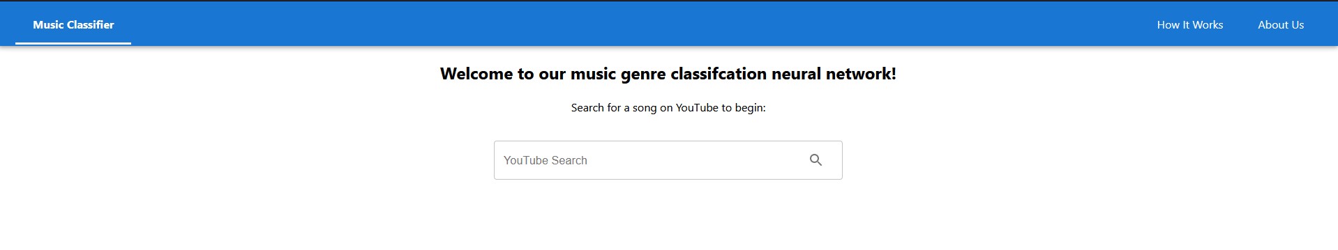
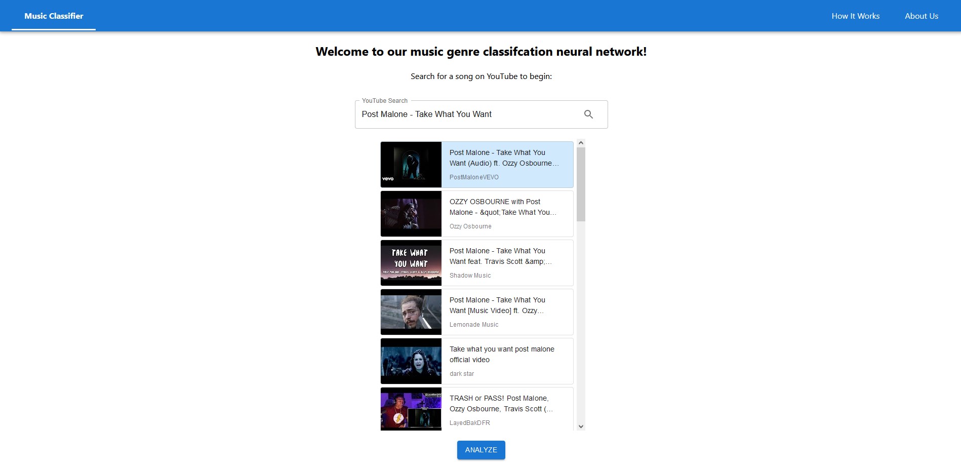
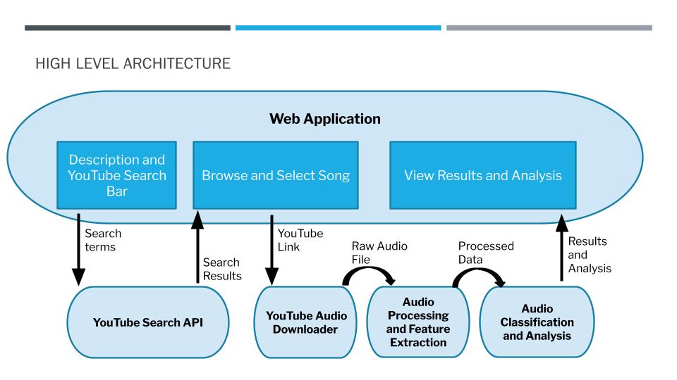
This project is a web application that allows users to search for a song on YouTube, select a song from a list of results, and receive a prediction for the music genre of the selected song.

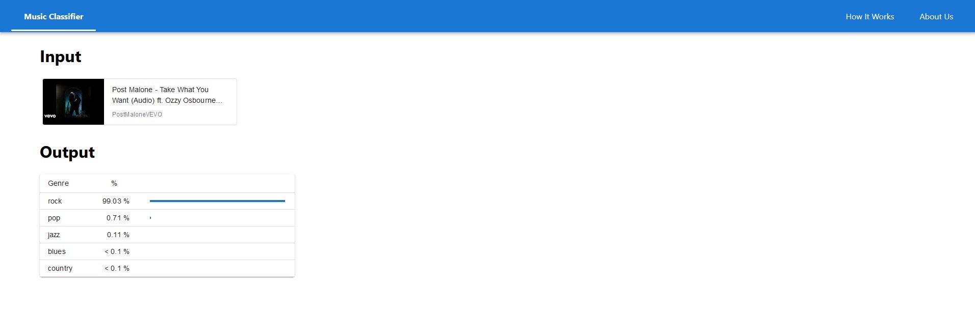
The model generates confidence scores for each of the 10 genres. The genre with the highest confidence score will be the prediction made. The top-5 confidence scores and the resulting genres are also displayed in addition to the top prediction on the webpage.

In addition to interacting with the ML model, users can visit the ‘How It Works’ page to get a more in depth discussion on how the model was trained and designed. The user can also visit the ‘About Us’ page to get information on the creators of the webpage.

You can access the website here or run it locally.

1. Install yarn if it isn't already installed: npm install yarn.
2. From the /frontend folder, run yarn start through the terminal.

1. Install flask if it isn't already installed: pip install Flask.
2. From the /api folder, run flask run --no-reload through the terminal.

UI Mockups: Figma

Language: Typescript

Framework: Create React App / React

UI Framework: Material UI

Language: Python

Framework: Flask

Libraries: Librosa, FFmpeg, youtube-dl

We deployed our application using Google Cloud, specifically the App Engine service. We set up separate front and back end services that allowed us to iterate and deploy those two codebases independently.

Language: Python

Libraries: Librosa, numpy, sklearn, tensorflow, keras

The GTZAN dataset was used for our dataset, which consists of 1000 .wav format audio tracks 30 seconds in length. To increase the size of the dataset, each audio track was split into 10 segments, each 3 seconds in length. Librosa was used to extract the Mel Spectrogram features from the audio segments. These features were then used to train a CNN model based on the AlexNet architecture using sklearn and tensorflow.keras. Using sklearn and tensorflow.keras, the model was saved and then used later for making predictions.

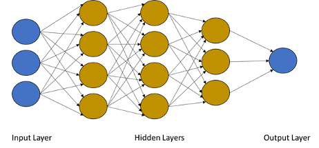
An artificial neural network loosely models a collection of neurons, such as those found in our brains. In the brain, a neuron can transmit an electrical signal to another neuron. This is modeled in an artificial neural network, commonly referred to as a neural network, as a graph. The connection between one neuron to another one is represented by an edge which is typically weighted. These weights are updated during the training of the network via mathematical equations. The network is split into layers consisting of a group of neurons. The network starts with an input layer, and will traverse through additional hidden layers, and finishes at an output layer. After training, a machine learning model is produced. Below is an example of a simple neural network architecture:

To train a neural network, training examples are needed. The training examples are typically in the form of datasets that consist of a collection of data that is related. For example, the MNIST is a dataset that consists of a total of 70,000 handwritten digit images.

For our project, we needed audio data to train a neural network to make music genre predictions. We used the GTZAN dataset that consists of 1000 .wav format audio tracks that are 30 seconds in length. The audio tracks are evenly split between 10 genres (100 audio tracks per genre): blues, classical, country, disco, hiphop, jazz, metal, pop, reggae, and rock.

In order to train an accurate model, many training examples are needed. When we learn a new skill, it often requires lots of practice in order to master the skill. The same concept applies in machine learning. GTZAN is considered a small dataset. To increase the number of training examples, the audio tracks were split into 10 segments, each consisting of 3 seconds in length. While 3 seconds may seem like a short amount of time, research suggests that the brain can recognize a familiar song in less than a second. Splitting the audio tracks into 10 segments created a new dataset that was approximately 10 times the size of the original GTZAN dataset.

You can download the GTZAN dataset and then run the Python script feature_extraction_dataset.py in the scripts folder from the GitHub repository to recreate this dataset.

To train a neural network, the architecture for the model must be designed as well as the equations that will be used for the connections between the different layers. One very popular model architecture is called AlexNet. AlexNet was developed in 2012 and is considered a convolutional neural network (CNN). In a CNN, the convolutional layers have filters that slide over the input features and produce feature maps. These layers make them ideal to use when processing 2-dimensional images, and as a result, CNNs are very popular with image classification/recognition models. For our project, we started with the AlexNet architecture and then modified it to fit the needs of the project.

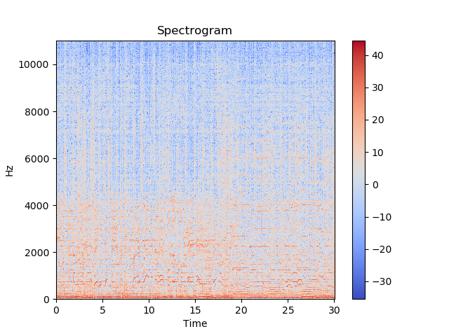
A question that may come to your mind is, why are we using a CNN for audio if it is best suited for images? For our dataset, we decided to use the mel spectrogram features of an audio sample to train our model. Sound can be thought of as a sequence of vibrations that changes in pressure strength. Imagine striking the key on a piano. Initially, the sound is loud but as time passes the sound becomes softer until it's completely silent. We can visualize this by plotting the pressure strength versus time to obtain a 2-dimensional image. We can add more detail by splitting the audio into small time windows and applying Fourier transforms to decompose the audio into frequencies. By combining all these time windows, a heat map can be produced that will display the time versus the frequencies with a color scale that represents the amplitude. Generally, the frequency is changed to a log scale and the color will be changed to decibels to produce a more visual friendly graph. This is known as a spectrogram as shown below:

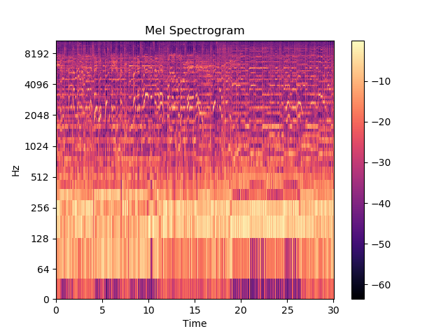
We'll further transform our data by using the Mel scale. Two sounds that are equal distance to one another on the Mel scale, should also be equal distance when perceived by a human. By applying this scale to our spectrogram, we can produce a Mel spectrogram, as seen below:

To train our model, we will feed these Mel spectrogram images into the model. The AlexNet architecture was used as the basis for our model, consisting of 5 convolutional layers and 3 fully connected layers (where all the inputs from the layer are connected to the activation unit of the next layer). An activation unit is a node that will implement the activation function, which is the function responsible for transformation. For AlexNet, this activation function is a rectified linear activation function (ReLU) that will output the value without change if it is positive and zero for any non-positive value.

After training, the model was around 200MB in size. However, GitHub only allows for files up to 100MB to be hosted. In order to reduce the storage requirements of our model, parts of the AlexNet architecture were removed or modified. We reduced the size and number of layers in our model and in the end, our model consisted of 4 convolutional layers and only 2 fully connected layers. The overall size of our model is approximately 24MB. The complete model architecture is given in the train_neural_network.py file in the scripts folder of our GitHub repository.

The accuracy of a model is often reported as a sign of how well the model performs. To calculate the model accuracy, we first use a set of training examples that the model has not seen before and then take the number of correctly predicted music genres divided by the total number of examples seen to get the accuracy. Our model’s accuracy on our test dataset was 75%.

To use our model for predictions on new audio files, the audio files must first be preprocessed. On the website, you will select a song from YouTube. The audio from that video is then downloaded and a 3 second clip of that audio is sampled. The Mel spectrogram features are then extracted and fed into the model. The prediction is made by using the final weights from training to produce the outcome. The model will generate confidence scores for each of the 10 genres. The genre with the highest confidence score will be the prediction made.

For our project, we list the top 5 confidence scores and their corresponding genres. The top 5 confidence scores are helpful to determine if the model is making a confident prediction. For example, an audio file that produces a top confidence score of 95% for a specific genre means that the model is very confident that the audio file is this genre. If an audio file has a top confidence score under 70%, then the model is not very confident in its prediction. In some cases, the model’s top confidence score may be below 50%.