Exploration of various neural network architectures that perform image denoising.
This data comes from a kaggle dataset. It contains chest x-ray images of individuals with and without pneumonia.
The best performing model was a residual autoencoder neural network. It has symmetric skip-forward connections between convolution layers of the same feature tensor shape. Hyperparameter tuning for this neural network architecture was conducted using random search. An example of the denoising performance of this model is shown below on a test-set image.
Noise is information that is not part of a desierd signal. For x-ray images, noise in the image can be caused by measurement errors or efforts to reduce patient's exposure to radiation. Denoising is often required for proper diagnostic analysis by medical professionals. Competent denoising software exists on the market, but there is still research interest due to:
- limited datasets for niche domains...specific diseases that don't have huge sample sets available (e.g. COVID-19)
- extreme cases of noisy images that software cannot handle
- limited applicable use cases for software
We will explore neural network models that perform image denoising on x-ray images of chest x-ray images. The dataset includes clean x-ray images. In this study, we will corrupt the image with various types of noise to produce training data.
The first neural network architecture of interest are autoencoders. It is a bow-tie shape network that condenses an input into a low dimensional latent space and then expands it out into an output that is similar to the input. This architecture excels that captures latent information about the domain of inputs and excluding any noise. Noise can be isolated by the loss function that compares the inputs to the outputs of the model.
encoder = tf.keras.Sequential([
        tf.keras.layers.InputLayer(input_shape=(64, 64, 1)),
        tf.keras.layers.Conv2D(filters=32, kernel_size=3, strides=(2, 2), activation='relu'),
        tf.keras.layers.Conv2D(filters=64, kernel_size=3, strides=(2, 2), activation='relu'),
        tf.keras.layers.BatchNormalization(),
        tf.keras.layers.Flatten(),
        # No activation
        tf.keras.layers.Dense(LATENT_DIM)
        ])

decoder = tf.keras.Sequential([
        tf.keras.layers.InputLayer(input_shape=(LATENT_DIM,)),
        tf.keras.layers.Dense(units=8*8*32, activation=tf.nn.relu),
        tf.keras.layers.Reshape(target_shape=(8, 8, 32)),
        tf.keras.layers.Conv2DTranspose(filters=64, kernel_size=3, strides=4, padding='same',
            activation='relu'),
        tf.keras.layers.Conv2DTranspose(filters=32, kernel_size=3, strides=2, padding='same',
            activation='relu'),
        # No activation
        tf.keras.layers.Conv2DTranspose(filters=1, kernel_size=3, strides=1, padding='same'),
        ])
Below is the model run aginst a test set image.

The variational autoencoder (VAE) is a variant of the autoencoder architecture. Instead of a latent dimension space of d, the variation autoencoder produces 2*d latent variables. These variables are parameters to a probabalistic function that represents the actual latent features. Thus, the 2*d parameters are used to sample d parameters that are then passed through the decoder. This architecture has more success in generative modeling since it attempts to model the probability distribution of the latent space instead of the values of the latent space directly. Because of this, random numbers within a given range are more agreeable with the decoder.
The last layer of the encoder is:
tf.keras.layers.Dense(LATENT_DIM + LATENT_DIM)
Additional sampling functions are created to complete the connection between the encoder and decoder. The sampling has no effect on backprop.
Below is a gif that shows generated images using randomly sampled numbers passed through the sampler and then the decoder at various epochs during training. The result is an image that somewhat shows how well the model has 'understood' the domain or captured the true latent features. This is not useful for denoising, just a fun graphic.
The VAE produces more smoothed images than the autoencoder. The performance appears to be similar to that of the regular autoencoder.

An autoencoder architecture with skip-forward connections was implemented using the tf.keras API. The skip-forward connections allow for better behavior during model training for very deep networks. Essentially, the activation of a particular layer is shortcutted further down the network. In this case, we implemented an identify residual skip-forward connection. If necessary, the residual block is able to learn the identity function and this helps stabalize training for large networks. This is of particular interest for our image denoising problem because we want to balance between having the network learn the complex meta-model of chest x-ray images (complex network architecture) but also possibly minimally adjust the values of certain pixels that experienced less noise (skip-connections).
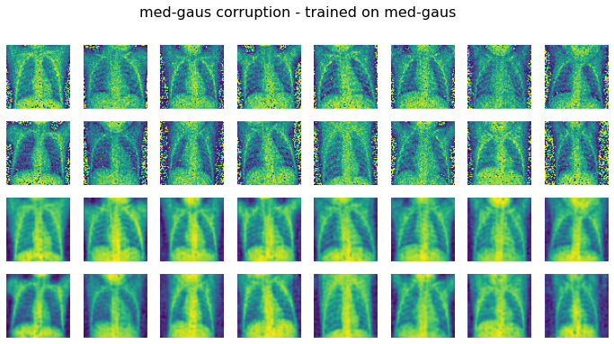
Random sampling was used to determine a good set of hyperparameters. The model was trained on a dataset corrupted by medium-level Gaussian noise. The performance of this model on a test set image is shown below. Overall, the denoising is much more successful than previous iterations. E.g. the rib cage is better denoised.
Below that is the performance of this model on different corruption types. The top two rows are the images with corruption. The bottom two rows of each figure are the denoised images corresponding to the corrupted image 2 rows above.


