- 1 Introduction
- 2 The Characteristic Function Route to Implied and Local Volatility
- 3 Monte Carlo
- 4 Using The Ito Language To Investigate Exotic Pricing
Vollab (Volatility Laboratory) is a python package for testing out different approaches to volatility modelling within the field of mathematical finance. The package is free to use for academic and research purposes. For any related commercial applications you are recommended to consult with the author. Notebooks demonstrating use of the Ito language for investigating the prices of exotics are now included.
Vollab contains an implementation of the Fast Fourier Transform method of Carr and Madan for calculating the prices of European call options, for stochastic processes with known characteristic function. Characteristic functions for Geometric Brownian Motion (Black-Scholes) and Heston’s stochastic volatility model are provided.
The figure below illustrates call prices produced using FFT for the Heston model.
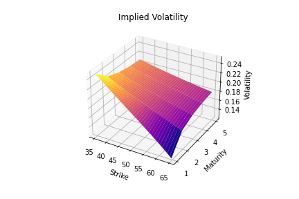
After production of call prices, Jackel’s "Lets Be Rational" methodology can be used to rapidly convert call prices to the implied volatility surface.
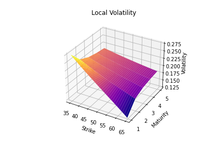
Finally implied volatility can be transformed to local volatility using Dupire’s formula.
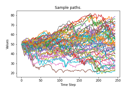
Vollab contains Monte Carlo samplers, for Geometric Brownian Motion (Black-Scholes), Heston’s stochastic volatility model and Local Volatility. One use of the samplers is to estimate prices by expectation in the appropriate probability measure.
The listing below defines an example of an exotic product in the Ito language, the Locally Capped Globally Floored Cliquet
# Mediobanca Bond Protection 2002-2005, ISIN IT0003391353
#
# Locally Capped Globally Floored Cliquet
#
underlying = "STOXX";
#
minCoupon = 0.02;
#
currency = "EUR";
#
notionalAmount = 1.0;
#
get notionalAmount * coupon[1] in currency on couponDates[1];
get notionalAmount * coupon[2] in currency on couponDates[2];
get notionalAmount * coupon[3] in currency on couponDates[3];
#
coupon[c] = max[sumReturns[c], minCoupon];
#
sumReturns[c] = sum[resetReturns[endDates[c], startDates[c]]];
#
resetReturns[{}, {}] = {};
resetReturns[t:ts, tm:tms] = min[max[r[t, tm], -0.01],  0.01] : resetReturns[ts, tms];
#
r[t, tMinus] = performance[s[t], s[tMinus]];
#
performance[st,stMinus] = (st - stMinus) / stMinus;
#
s[t] = Observe[underlying, t];
#
startDates[c] = dropTail[resetDates[c]];
#
endDates[c] = dropHead[resetDates[c]];
#
couponDates[1] = '2002-12-02';
couponDates[2] = '2003-12-02';
couponDates[3] = '2004-12-02';
#
resetDates[1] = {
'2002-01-02',
'2002-01-02',
'2002-02-02',
'2002-03-02',
'2002-04-02',
'2002-05-02',
'2002-06-02',
'2002-07-02',
'2002-08-02',
'2002-09-02',
'2002-10-02',
'2002-11-02',
'2002-11-25'};
#
resetDates[2] = {
'2003-01-02',
'2003-01-02',
'2003-02-02',
'2003-03-02',
'2003-04-02',
'2003-05-02',
'2003-06-02',
'2003-07-02',
'2003-08-02',
'2003-09-02',
'2003-10-02',
'2003-11-02',
'2003-11-25'
};
#
resetDates[3] = {
'2004-01-02',
'2004-01-02',
'2004-02-02',
'2004-03-02',
'2004-04-02',
'2004-05-02',
'2004-06-02',
'2004-07-02',
'2004-08-02',
'2004-09-02',
'2004-10-02',
'2004-11-02',
'2004-11-25'
};
#
# remove the head (first entry) from the list
dropHead[{}] = {};
dropHead[{x}] = {};
dropHead[x:xs] = xs;
# remove the tail (last entry) from the list
dropTail[{}] = {};
dropTail[{x}] = {};
dropTail[x:xs] = x : dropTail[xs];
# minimum of two numbers.
min[x,y] = if x < y then x else y endif;
# maximum of two numbers.
max[x,y] = if x < y then y else x endif;
# sum of a list of numbers
sum[{}] = 0;
sum[{x}] = x;
sum[x:xs] = x + sum[xs];
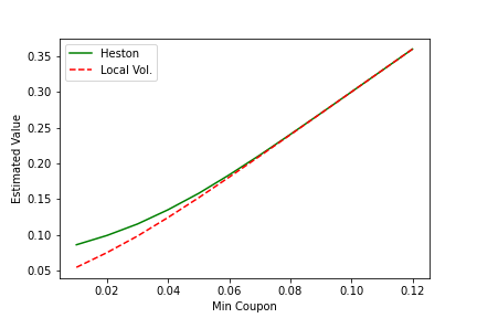
Two different models that match the prices of plain-vanilla options can give quite different prices for exotics. This is commonly summarised by stating exotics can be forward skew dependent. The notebooks make use of the Ito language to demonstrate these differences. The figure below illustrates the divergence in price as a function of the "Min Coupon" parameter, between the Heston model and Local Volatility. For more about exotics see the discussion in, "The volatility surface: a practitioner’s guide".


