Disclaimer: below some ramblings on methods development for BEAST 2 [@beast, @beastbook, @bouckaert2019beast] packages. This is a living document based on collected wisdom of BEAST developers, which keeps evolving.
This document is about testing validity of a BEAST method, not the programming aspects (like setting up dependencies, wrapping up files into a package, etc.), which can be found in the tutorial for writing a BEAST 2 package and writing a package for a tree prior tutorial.
There are several levels of validation:
- the model appears to produce reasonable results on a data set of interest.
- the model produces more reasonable results on a data set of interest than other models.
- unit tests show correctness of direct simulator implementation, likelihood implementation and/or operator implementation(s).
- sampling from prior conforms to expectations.
- a simulation study shows parameters simulated under the model can be recovered by inference from simulated data for a fixed tree and fixed other parameters for a small number of illustrative cases.
- as previous but with sampled tree and sampled parameters, so the process is repeated
$N$ times and tree and parameters sampled from a reasonable prior. - a simulation study shows the model can recover parameters (most of the time) even when there are model violations in simulating the parameters.
Automate the experiment -- you will do it again, in about 6 months time, when you least expect it.
Document the experiment -- "It is like cleaning toilets: nobody want to do it, but it is more pleasant for visitors. You will probably be one of those visitors in 6 months time..."
http:https://videolectures.net/cancerbioinformatics2010_baggerly_irrh/
Reproducibility with docker:
Steps to run the attached BEAST 2 analysis:
- Install Docker (www.docker.com)
- From a terminal window, run the following from the directory containing the XML file:
docker run -v$PWD:/data tgvaughan/beast2_bacter beast ecoli.xmlThat's it! (Under Windows the $PWD would have to be replaced with the path of the current directory.) These instructions are impervious to most things we worry about: core and package API changes, Java version changes and OS dependencies.
New methods require usually require two parts: an implementation
- the simulator implementation
$S(M)\to\theta$ (if any) - the model implementation
$I(M)$ - operator implementations
$R$
To verify correctness of a simulator implementation
When no analytical estimates of statistics are available, it may be possible to find a simplified case for which an analytical solution exists, for example when the tree only has two taxa.
Examples of simulators (this list is far from exhaustive):
- the MASTER [@vaughan2013stochastic] BEAST 2 package is a general purpose package for simulating stochastic population dynamics models which can be expressed in terms of a chemical master equation.
- SimSnap for SNAPP [@bryant2012inferring] is a custom build implementation in C++ for simulating alignments for a fixed tree and SNAPP parameters.
- The
beast.app.seqgen.SequenceSimulatorclass in BEAST 2 can be used to simulate alignments for general site models using reversible substitution models. See testSeqGen.xml for an example. - Models implemented in other phylogenetic software packages, such a BEAS 1, MrBayes, RevBayes, allow sampling a distribution using MCMC.
- The
beast.core.DirectSimulatorclass in BEAST 2 can be used to draw samples from distributions in BEAST that extendbeast.core.distribution.Distributionand implement thesample(state, random)method. You can set up an XML file and run it in BEAST. Here are a few examples: testDirectSimulator.xml, testDirectSimulator2.xml, and testDirectSimulatorHierarchical.xml.
For small examples for which an analytical result can be calculated a unit test can be written to confirm the implementation behaves correctly for the expected result. For example, for a small tree ((A:1.0,B:1.0):1.0,(C:1.0,D:1.0):1.0) with birth rate 1 we can calculate the expected value of the Yule prior (
package test;

import org.junit.Test;

import beast.evolution.speciation.YuleModel;
import beast.util.TreeParser;
import junit.framework.TestCase;

public class YuleLikelihoodTest extends TestCase {

	@Test
	public void testYuleLikelihood() {
        TreeParser tree = new TreeParser("((A:1.0,B:1.0):1.0,(C:1.0,D:1.0):1.0);");

        YuleModel likelihood = new YuleModel();
        likelihood.initByName("tree", tree, "birthDiffRate", "1.0");

        assertEquals(-6.0, likelihood.calculateLogP());
    }

}
In theory, the inferred distributions
The Hastings ratio for this operator is
In BEAST, if the sample method is implemented in a class derived from Distribution, you can use beast.experimenter.DirectSimulatorOperator in the Experimenter package to set up an MCMC analysis in XML. Here is an example that draws a birth rate from an exponential distribution with mean 1, and a Yule distribution to generate a tree. Note that the tree heigh statistic is logged, as well as an expression for a clock rate (being 0.5/tree-height) for evaluation purposes. The MCMC sample can be compared with the direct sample using the example file testDirectSimulator.xml.
<beast version="2.0" namespace="beast.core
:beast.evolution.alignment
:beast.evolution.tree
:beast.math.distributions
:beast.evolution.speciation
:beast.core.util
:beast.core.parameter">


    <run spec="MCMC" chainLength="1000000">
    	<state id="state">
    		<stateNode idref="tree"/>
    		<stateNode idref="birthDiffRateParam"/>
    	</state>

        <distribution spec="CompoundDistribution" id="fullModel">
            <distribution spec="YuleModel" id="yuleModel">
                <tree spec="Tree" id="tree">
                    <taxonset spec="TaxonSet">
                        <taxon spec="Taxon" id="t1"/>
                        <taxon spec="Taxon" id="t2"/>
                        <taxon spec="Taxon" id="t3"/>
                        <taxon spec="Taxon" id="t4"/>
                        <taxon spec="Taxon" id="t5"/>
                    </taxonset>
                </tree>
                <birthDiffRate spec="RealParameter" id="birthDiffRateParam" value="1.0"/>
            </distribution>

            <distribution spec="beast.math.distributions.Prior" id="birthDiffRatePrior">
                <distr spec="Exponential" id="xExpParamDist" mean="1"/>
                <x idref="birthDiffRateParam"/>
            </distribution>

        </distribution>

		<operator spec="beast.experimenter.DirectSimulatorOperator" weight="1" state="@state">
			<simulator id="DirectSimulator" spec="beast.core.DirectSimulator" nSamples="1">
				<distribution idref="fullModel"/>
			</simulator>
		</operator>

        <logger id="tracelog" logEvery="1000" fileName="$(filebase).log">
            <log idref="birthDiffRateParam"/>
            <log id="clockRate" spec="beast.util.Script" expression="0.5/TreeHeight">
            	<x id="TreeHeight" spec="beast.evolution.tree.TreeHeightLogger" tree="@tree"/>
            </log>
            <log idref="TreeHeight"/>
        </logger>

        <logger id="treelog" logEvery="1000" fileName="$(filebase).trees">
            <log idref="tree"/>
        </logger>

        <logger id="screenlog" logEvery="1000">
            <log idref="birthDiffRateParam"/>
        </logger>
    </run>
</beast>
Make sure when sampling from the prior through MCMC that the chain length is sufficiently large and log frequency large enough to ensure that each sample is independent of the previous sample. The ESSs shown in Tracer should be close to N when there are N samples in the trace log, for most of the items in the log. There may be a few items with an ESS that is a bit lower, and inspection of the trace plot should tell you whether lower log frequencies should be used.
Comparing two distributions can be done by
- eye balling the marginal likelihoods in Tracer and making sure they are close enough.
- testing whether parameters are covered 95% of the time in the 95% HPD interval of parameter distributions.
- using a statistical test, e.g. the Kolmogorov-Smirnov test, to verify the distributions
$p_I(\theta|M)$ and$p_S(\theta|M)$ are the same.
TraceKSStats calculate Kolmogorov-Smirnof statistic for comparing trace logs. TraceKSStats has the following inputs:
- trace1 (LogFile): first trace file to compare (required)
- trace2 (LogFile): second trace file to compare (required)
- burnin (Integer): percentage of trace logs to used as burn-in (and will be ignored) (optional, default: 10)
Sample output:
Trace entry                                      p-value
posterior                                        1.0
likelihood                                       0.21107622404022763
prior                                            0.036794035181748064
treeLikelihood                                   0.04781117967724258
TreeHeight                                       0.036794035181748064
YuleModel                                        0.005399806065857771
birthRate                                        0.2815361702146215
kappa                                            0.62072545444263
freqParameter.1                                  0.0
freqParameter.2                                  8.930072172019798E-5
freqParameter.3                                  1.0883734952171764E-6
freqParameter.4                                  0.0
Though some values have very low p-values, meaning they differ significantly, it is recommended to verify this using Tracer to make sure that the test is not unduly influenced by outliers.
If you have an implementation of a model that shows up in a profiler as being time consuming, it may be worth spending time to improve the computational efficiency of the model. To verify correctness of the new model you can just add both implementations to the likelihood or prior (whatever is appropriate) in the XML and log both of them. If they show different values in the log that is evidence something different is happening in the new implementation.
Obviously, it will be sampling from a more peaked distribution since the contribution of the model is counted twice, but if correctness is what you are interested in this would work.
Makes sure to log with frequency << 10000, since every 10000 steps these likelihoods will be calculated from scratch.
For a density
$$ E(U(\theta,x)) = \int U(\theta,x)p(x;\theta)dx = 0 $$ {#eq:scorefunction}
(this is the expected value over the data
$$ E\left(U(\theta, x)U(\theta, x)^T + {\partial^2}/{\partial\theta^2}\ \log p(x;\theta)\right) = 0 $$ {#eq:variancestatistic}
These properties can be used in conjunction with a direct simulator as a necessary but not sufficient check that the likelihood is implemented correctly. The score function (+@eq:scorefunction) and Hessian (+@eq:variancestatistic) statistics can be calculated on samples from the simulator and a hypothesis test used to check that their mean is 0. In the multivariate case a potentially useful test is the likelihood ratio test for a multivariate normal with zero mean (implemented here). If there are non-identifiable parameters there may be issues with performing this test as colinearity will lead to a singular sample covariance matrix.
In practice it is appropriate to compute the score function by calculating derivatives using finite differences (implemented here).
The BEAST validation package is designed around three core object types: it performs a test on statistics drawn from samplers.
BEAST validation tests are implemented within the BEAST 2 XML parser framework. The main Runnable class is beast.validation.StochasticValidationTest. StochasticValidationTest has inputs for each of the core object types: samplers, statistics and a test. Note that some tests may be designed for one, two or many sampler/statistic pairs.
StochasticValidationTest has some additional parameters:
alpha: The significant level to use in the testnSamples: The number of samples to draw from each samplerprintEvery: How often to report sampling progresssampleLoggers: Loggers to run for every sample (usually the statistics)resultLoggers: Loggers to run after testing
There are currently two useful combinations of samplers, statistics and test implemented by BEAST validation.
This test validates a combination of likelihood and direct simulator using a known property of probability density functions: that the expectation of the gradient of the log-likelihood at the true parameter values is zero (see stats-tricks.md). The core components of this test are (with a single sampler-statistic pair):
- a simulator: This could be a custom simulator, or make use of one of the generic simulation tools available, such as
beast.simulation.TreeSamplerFromMaster beast.validation.statistics.NumericalScoreFunctionStatistics: a statistic that uses a finite differences to calculate the gradient of a likelihood with respect to some parameters- Note that the
RealParameterobjects included in theparameterinput should be the same provided to theDistributionin thelikelihoodinput
- Note that the
beast.validation.tests.MultivariateNormalZeroMeanTest: a likelihood ratio test that uses a multivariate normal fit to the gradients to test for zero mean
An important note is that there are some regularity conditions on the parameters you can use in this test. Roughly, they must not affect the support of the data, which excludes the origin time parameter in tree priors. See stats-tricks.md for further details.
An example XML for this test on the birth-death-sampling tree prior can be found in the BEAST validation examples.
Once you have created an XML and installed the BEAST validation package (pending inclusion in the package repository) using the standard BEAST 2 launcher. Once your test has run, it will provide the result on the console:
Performing test...
Test PASSED
p value: 0.284784
Once simulator
The direct simulator operator (see DirectSimulatorOperator above) can be used as starting operator, and new operators added one by one to verify correctness.
The BEAST 2 Experimenter package can assist (see section "Using the Experimenter package" below).
A useful test for an MCMC sampler for a model (likelihood + operators) is if it can produce the same distribution as direct simulation. For phylogenetic models, this would usually be the tree prior. The core components of this test:
- Two samplers
- a simulator (see the previous test for details)
beast.core.SamplerFromMCMC- extends the normal BEAST MCMC class
- needs a model/likelihood and operators
- To test a single, potentially non-ergodic operator, a separate simulator could be used as a global operator with the
beast.simulation.OperatorFromSamplerclass
- A multivariate statistic
beast.validation.statistics.UltrametricTreeStatisticsprovides some basic statistics on BEAST time trees- For an example of statistics on more complex tree-like objects, see
bacter.util.ConversionGraphStatsLogger
beast.validation.tests.BootstrapMultivariateDistributionTest: a test that bootstraps a multivariate generalisation of the Kolmogorov-Smirnov (KS) statistic to compare distributions (see [stats-tricks.md] for further details)
An example XML for this test on the birth-death-sampling tree prior can be found in the BEAST validation examples.
If you see this error message during an MCMC run, there probably is an error in the way that a CalculationNode in your model is caching its state. More information is on the beast site blog post.
One way to hunt down this error is by using checksums on calculation nodes (thanks Nico!). Code in the inner loop of the MCMC class is only executed when the debugFlag is set, which happens when running java with -Dbeast.debug=true.
At the start of an iteration of the MCMC, we store a checksum of each CalculationNode If the step is rejected, we check whether all the checksums are equal to the stored ones.
If the checksums are not the same, clearly something went wrong when trying to restore the previous state and we throw an exception. There are (at least) two reasons why this might happen:
- The store/restore methods are incorrect or missing.
- A fat
CalculationNodewas changed in an operator proposal, beforestore()is called (this may be particularly hard to find).
In the current implementation the checksum method defaults to returning a constant 0, which means no exceptions will be thrown. Furthermore the checks are only performed when the debugFlag is set. Hence, check sum calculation will not interfere with running analyses. BEAST2 developers who want to use the checks can override the getChecksum() method for the StateNodes and fat CalculationNodes they want to check.
Here are two example implementations:
Tree checksum -- as a simple checksum for the Tree class we could take a hash value of the root height:
    @Override
    public int getChecksum() {
        return Double.hashCode(getRoot().getHeight());
    }
However, bugs that don't affect the root height could still slip through and we could make the test more elaborate by hashing all heights and information about the topology as well.
TreeLikelihood checksum -- in the case of the tree likelihood we can simply use a hash value of getCurrentLogP() as a checksum:
    @Override
    public int getChecksum() {
        return Double.hashCode(getCurrentLogP());
    }
In summary:
- use Bactrian kernels if you can (currently in the BEASTLabs package).
- use AdaptableOperatorSampler from the ORC package if you have multiple
See blog post for details.
Using the direct simulator can be done as follows
- Set up
DirectSimulatorat top level - Add model to simulate from
- Add loggers to register output
Use the nSamples attribute to specify how many samples to draw.
<beast version="2.0" namespace="beast.core:beast.evolution.alignment:beast.evolution.tree:beast.math.distributions:beast.evolution.speciation:beast.core.util:beast.core.parameter">

    <run spec="DirectSimulator" nSamples="100">

		<!-- model goes here -->

		<!-- loggers go here -->

    </run>
</beast>
Here, the model consists of a birthDiffRate parameter, drawn from an exponential distribution. This rate is used in a Yule model to draw trees over a set of 5 taxa, called t1, t2,...,t4. This is placed inside the run element above.
<distribution spec="CompoundDistribution" id="fullModel">
    <distribution spec="YuleModel" id="yuleModel">
        <tree spec="Tree" id="tree">
            <taxonset spec="TaxonSet">
                <taxon spec="Taxon" id="t1"/>
                <taxon spec="Taxon" id="t2"/>
                <taxon spec="Taxon" id="t3"/>
                <taxon spec="Taxon" id="t4"/>
                <taxon spec="Taxon" id="t5"/>
            </taxonset>
        </tree>
        <birthDiffRate spec="RealParameter" id="birthDiffRateParam" value="1.0"/>
    </distribution>

    <distribution spec="beast.math.distributions.Prior" id="birthDiffRatePrior">
        <distr spec="Exponential" id="xExpParamDist" mean="1"/>
        <x idref="birthDiffRateParam"/>
    </distribution>
</distribution>
Since we sample a parameter and a tree, we need a trace log and a tree log. Appart from state nodes, other statistics can be sampled as well. For example, here, we log the height of the tree using a TreeHeightLogger, and log a clock rate suitable for the tree using the expression 0.5/TreeHeight using the Script class form the BEASTLabs package. The loggers should be placed inside the run element as well.
<logger logEvery="1" fileName="$(filebase).log">
    <log idref="birthDiffRateParam"/>
    <log id="TreeHeight" spec="beast.evolution.tree.TreeHeightLogger" tree="@tree"/>
    <log id="clockRate" spec="beast.util.Script" expression="0.5/TreeHeight">
    	<x idref="TreeHeight"/>
    </log>
</logger>

<logger logEvery="1" fileName="$(filebase).trees">
    <log idref="tree"/>
</logger>
The complete XML file can be found as testDirectSimulatorByMCMC.xml in the Experimenter package.
Conversion requires the following steps:
- replace top level run element by MCMC
- add state element and references to state nodes
- add
DirectSimulatorOperator - add screen logger (optional)
When you have meta data associated with branche of trees, like population sizes or clock rates, it is usually easy to verify that the meta data that is inferred is compatible for the leaf nodes. Leaf nodes are in a tree with
However, the branches that do not end in a leaf are numbered
One way to verify the correctness of estimates of metadata on branches is do a well calibrated simulation study that
- logs the tree + metadata used to generate the alignment.
- create a summary tree with topology equal to the generating tree.
- run
MCCTreeComparatorto summarise results.
In the BEAST XML template, add a tree logger that logs the tree used to generate the alignment, e.g like so:
    <logger id="sim.treelog.t:alignment" spec="Logger" fileName="sim.$(filebase).trees" logEvery="1000000000" mode="tree">
        <log id="sim.TreeWithMetaDataLogger.t:alignment" spec="beast.phoneme.BranchMetadDataLogger" tree="@sim.Tree.t:alignment">
        	<metadata idref="sim.permutation.s:alignment"/>
        </log>
    </logger>
We only need this to be logged once, to the logEvery value can be set very high.
Say, we stored the generating trees in files sim.analysis-0.trees, sim.analysis-1.trees, etc. numbered 0 through to 99. Treeannotator (part of BEAST) can be used to summarise trees and their metadata on the tree topology used to generate the data using the -target option. On unix-like systems, the following command will generate summary trees for each of the 100 runs:
for i in {0..99}; do
	treeannotator -b 10 -target sim.analysis-$i.trees analysis-$i.trees analysis-$i.tree
done
MCCTreeComparator is a tool that is part of the beast-validation package, which produces coverage summaries for branch metadata.
MCCTreeComparator has the following options:
- tree (TreeFile): source tree file with meta data (required)
- mcc (TreeFile): MCC source tree file (required)
- from (Integer): start value to loop over (optional, default: 0)
- to (Integer): end value (inclusive) to loop over. If less than 0, no loop is performed. If more than 0, the part $(n) in the file path will be replaced by an integer, starting at 'from' and ending in 'to' (optional, default: 99)
- out (OutFile): output file, or stdout if not specified (optional, default: [[none]])
The output is a small report containing coverage information for total, leaf branches and internal brances separately. For real valued metadata it is the percentage of clades where the generating value is in the 95% HPD that is estimated (like clade height). For categorical values (below p1, p2, p3 and p4) it is the percentage of clades where the generating value is in the 95% credible set. The height and posterior entries show an 'N/A' for not applicable for leaf branch matches.
| metadata | % matches | % leaf branch matches | % internal branch matches |
|---|---|---|---|
| height | 95 | N/A | 95 |
| p1 | 99.3 | 99.5 | 99 |
| p2 | 99.6 | 99.83 | 99.25 |
| p3 | 99.9 | 100 | 99.75 |
| p4 | 99.1 | 99.83 | 98 |
| posterior | 99.6 | N/A | 99.6 |
Validation only covers cases in as far as the prior covers it -- most studies will not cover all possible cases, since the state space is just to large. Usually, informative priors are required for validation to work, since broader priors (e.g. some of the default tree priors in BEAST) lead to identifiability issues, for example, due to saturation of mutations along branches of a tree.
The mutation rate
- for reasonable computation times, trees should be about 0.5 substitutions high, OR
- sequences should be very long to reliably reconstruct smaller trees.
One way to enforce this is by
- a narrow prior on birth rates (for birth/death type tree priors), or
- putting an MRCA prior on the height of the tree, for coalescent models. Note that the latter hampers direct simulator implementations.
For clock models with mean clock rate != 1, simulate trees with clock rates times tree height approximately 0.5. This can be enforced using a prior on the clock rate times tree height, like so (note that this does not work with direct simulator implementations):
<prior id="ClockPrior.t:dna" name="distribution">
    <x id="evodistance" spec="beast.util.Script" argnames="clock height" expression="clock * height">
    	<x idref="clockRate.c:dna"/>
    	<x id="height" spec="beast.evolution.tree.TreeHeightLogger" tree="@Tree.t:dna"/>
    </x>
    <LogNormal mean="0.5" sigma="0.05" name="distr" meanInRealSpace="true"/>
</prior>
Published mutation rates can range from
For releases, tree priors for clock and trees should be made less informative in order to cater for a wider range of tree heights and clock rates.
To prevent saturation, adding categories with slow rates will go some way to allow covering a larger range of clock rates. Using gamma rate heterogeneity with shape values in the range 0.1 to 1 allows this, so adopt a gamma shape prior accordingly.
Since each site evolves with non-zero rate, use of proportion invariable sites is modelling the process badly, and therefore not recommended.
Priors ideally should be set in realistic ranges, e.g. frequency priors not uniform(0,1) but Dirichlet(4,4,4,4) is better.
Default priors seem OK for most substitution models.
SequenceSimulator (alternatively SimulatedAlignment) can help generate individual alignments.
SequenceSimulatorcan be used to generate a static alignment that can be merged into existing XML (e.g. with the help ofbeast.app.seqgen.MergeDataWith).SimulatedAlignmentcan be used as replacement of an alignment in the XML and will generate a new alignment every time BEAST is started on the XML.
To generate N XML files, use CoverageTestXMLGenerator in Experimenter package
The sequence length should be long enough that trees can be reasonably reliably recovered -- if the difference between longest and shorted tree is 2 orders of magnitude, nucleotide sequences of 10 thousand sites. When
Make sure log files names do not overlap.
Use logFileName="out$(N).log and start BEAST with
for i in {0..99} do /path/to/beast/bin/beast -D N=$i beast$i.xml; done
One reason coverage can be lower is if the ESSs are too small, which can be easily checked by looking at the minimum ESS for the log entry. If these values are much below 200 the chain length should be increased to be sure any low coverage is not due to insufficient convergence of the MCMC chain.
When using empirical frequencies, these frequencies can bias estimates of other parameters (like gamma shape for gamma rate heterogeneity), causing low coverage for these parameters. Especially for short sequences, empirical estimates can be far away from the frequencies used to generate the data. For that reason, empirical frequencies should be avoided, and estimated frequencies used instead.
Another argument against empirical frequencies is that it is double dipping: using the data to both estimate frequencies and ....
The occasional 91 is acceptable (the 95% HPD = 91 to 99 probability the implementation is correct) but coverage below 90 almost surely indicate an issue with the model or operator implementation. Also, coverage of 100 should be looked at with suspicion -- it may indicate overly wide uncertainty intervals.
If correct, distributed binomial with p=0.95, N=100:
| k | p(x=k) | p(x<=k) | p(x>=k) |
|---|---|---|---|
| 90 | 0.0167 | 0.0282 | 0.9718 |
| 91 | 0.0349 | 0.0631 | 0.9369 |
| 92 | 0.0649 | 0.1280 | 0.8720 |
| 93 | 0.1060 | 0.2340 | 0.7660 |
| 94 | 0.1500 | 0.3840 | 0.6160 |
| 95 | 0.1800 | 0.5640 | 0.4360 |
| 96 | 0.1781 | 0.7422 | 0.2578 |
| 97 | 0.1396 | 0.8817 | 0.1183 |
| 98 | 0.0812 | 0.9629 | 0.0371 |
| 99 | 0.0312 | 0.9941 | 0.0059 |
| 100 | 0.0059 | 1.0000 | 0.0000 |
source https://www.di-mgt.com.au/binomial-calculator.html for different values of p and N.
- ESS too low
loganalyserwas called without*.loginstead ofout?.log out??.log out???.log. As a result, theloganalyseroutput and trace log of true values are in different order. Rerunloganalyserto make sure the output is in the right order.- improper priors used: all priors should be proper, that is integrate to 1. Examples of improper priors are the 1/X and uniform prior with infinite upper and/or lower bounds.
- priors are outside the range usually used in applying the model, especially the next case:
- trees cannot be reconstructed reliably (height should not be too small or large).
- Hastings ratio in operators incorrectly implemented
- bug in model likelihood
- For released software, default priors should be made as uninformative as possible and/or provide some guidance on how to set them -- users will use defaults.
- Make sure to consider a number of scenarios, e.g. for clock models, scenarios from setting up rates page on beast2.org.
When publishing well calibrated studies, all XML files, log files and scripts for manipulating them should be made available, so the study can be replicated exactly as is. A practical way to do this is through a github repository.
Version numbers of BEAST and packages used should be noted.
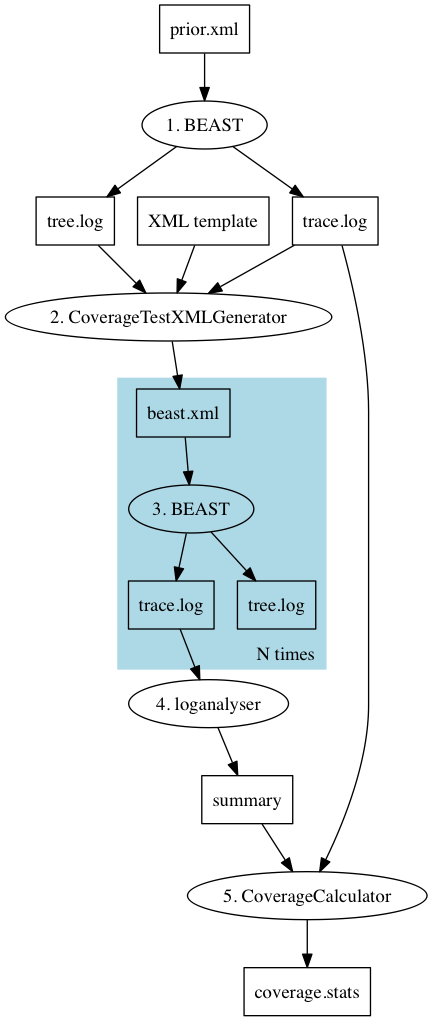
Experimenter is a BEAST 2 package that assists in simulation studies to verify correctness of the implementation. The goal of this particular simulation studies is to make sure that the model or operator implementation is correct by running N analysis on simulated data (using SequenceSimulator) on a tree and site model parameters sampled from a prior.
To run a simulation study:
- set up XML for desired model and sample from prior
- generate (MCMC) analysis for each of the samples (say 100)
- run the analyses
- use loganalyser to summarise trace files
- run
CoverageCalculatorto summarise coverage of parameters
Make sure to have the Experimenter package installed (details at the end).
First, you set up a BEAST analysis in an XML file in the configuration that you want to test. If you are using MCMC, set the sampleFromPrior="true" flag on the element with MCMC in it, and sample from the prior.
Alternatively, use a DirectSimulator as in this example: testDirectSimulator.xml.
Make sure that the number of samples in the trace log and tree log is the same and that they are sampled at a frequency such that there will be N useful samples (say N=100).
CoverageTestXMLGenerator2 Generate XML for performing coverage test (using CoverageCalculator). A template XML file should contain SimulatedAlignments with a tree, branch rate model and site model specified. These can be parameterised by using string of the form $(n) where n should match exactly the columns in the trace log file, or it can be $(tree) which is replaced by the species tree as specified in the -treeFile option. For individual gene trees use the -geneTreeFile option (detailed below). Example input files can be found here.
It has the following options:
- workingDir (File): working directory where input files live and output directory is created (optional)
- outDir (String): output directory where generated XML goes (as sub dir of working dir) (optional, default: mcmc)
- logFile (LogFile): trace log file containing model parameter values to use for generating sequence data (optional)
- treeFile (TreeFile): tree log file containing trees to generate sequence data on (optional)
- geneTreeFile (File): (optional) configuration file with gene tree identifiers and log file names, one per line separated by a tab,for example
gene1	/xyz/abc/gene1.trees
gene2	/xyz/abc/gene2.trees
In the XML, any instance of $(gene1) will be replaced by a tree from the file /xyz/abc/gene1.trees, and likewise for $(gene2).
- xmlFile (XMLFile): XML template file containing analysis to be merged with generated sequence data (optional)
- skip (Integer): numer of log file lines to skip (optional, default: 1)
- help show arguments
NB: make sure to set sampleFromPrior="false" in the XML.
NB: to ensure unique file name, add a parameter to logFileName, e.g.
logFileName="out$(N).log"
With this setting, when you run BEAST with -D N=1 the log file will be out1.log.
NB each SimulatedAlignment should have its own tree, sitemodel and branch rate mdoel, and should not share any of them with the remaining XML. This ensures that the start state and actual parameter values used to generate alignments are independent. If the true state and start state are the same, the analysis may be biased towards
Alternative Step 2. Generate (MCMC) analysis for each of the samples (support for multiple alignments)
Instead of generating complete BEAST XML files, including alignments, XML files can be generated where the state is initialised by start values from the trace log and the tree is initialised with trees from the tree log in Newick format through TreeParser. The alignment can then be generated on the fly with the help of beast.app.seqgen.SimulatedAlignment. Note that every time BEAST is started on the XML a new alignment will be generated, and unless the same seed is used, these alignments will be unique (almost surely).
Use your favourite method to run the N analyses, for example with a shell script
for i in {0..99} do /path/to/beast/bin/beast -D N=$i beast$i.xml; done
where /path/to/beast the path to where BEAST is installed.
Use the loganalyser utility that comes with BEAST in the bin directory. It is important to use the -oneline argument so that each log line gets summarised on a single line, which is what CoverageCalculator expects. Also, it is important that the log lines are in the same order as the log lines in the sample from the prior, so put the results for single digits before those of double digits, e.g. like so:
/path/to/beast/bin/loganalyser -oneline out?.log out??.log > results
where out the base name of your output log file.
NB if loganalyser is called with `out*.log`, results may end up in order `1,10,11,...,19,2,20,21,...` because file systems order items alphabetically. This makes matching with the true values impossible.
You can run CoverageCalculator using the BEAST applauncher utility (or via the File/Launch Apps meny in BEAUti).
CoverageCalculator calculates how many times entries in log file are covered in an estimated 95% HPD interval and has the following arguments:
- log
<filename>log file containing actual values - skip
<integer>numer of log file lines to skip (default: 1) - logAnalyser
<filename>file produced by loganalyser tool using the -oneline option, containing estimated values - out
<directory>output directory for tsv files with truth and estimated mean and 95% HPDs, and directory is also used to generate svg bargraphs and html report. Not produced if not specified. -excludex,y,zcomma separated list of entries to exclude from the analysis. By default,posterior,priorandlikelihoodare excluded. - typeFile (File): if specified, the type file is a tab delimited file with first column containing entry names as they appear in the trace log file, and second column variable type, d for double, b for binary, c for categorical, for example:
variable		type
birthRate		d
kappa			d
hasGamma		b
modelIndicator	c
Items that are not specified are considered to be of type double.
It produces a report like so:
                                                coverage Mean ESS Min ESS
posterior                                       0	   2188.41  1363.02
likelihood                                      0	   4333.99  3042.15
prior                                           33	   1613.20  891.92
treeLikelihood.dna                              0	   4333.99  3042.15
TreeHeight                                      95	   3076.44  2233.29
popSize                                         94	   577.20  331.78
CoalescentConstant                              91	   1620.76  787.30
logP(mrca(root))                                97	   4320.70  3328.88
mrca.age(root)                                  95	   3076.44  2233.29
clockRate                                       0	   3046.64  2174.60
freqParameter.1                                 98	   4332.76  3388.90
freqParameter.2                                 97	   4337.93  3334.29
freqParameter.3                                 96	   4378.30  3462.73
freqParameter.4                                 92	   4348.83  3316.36
Coverage should be around 95%. One reason coverage can be lower is if the ESSs are too small, which can be easily checked by looking at the Mean ESS and Min ESS columns. If these values are much below 200 the chain length should be increased to be sure any low coverage is not due to insufficient convergence of the MCMC chain. The occasional 90 or 91 is acceptable but coverage below 90 almost surely indicate an issue with the model or operator implementation.
The values for posterior, prior and treelikelihood can be ignored: it compares results from sampling from the prior with that of sampling from the posterior so they can be expected to be different.
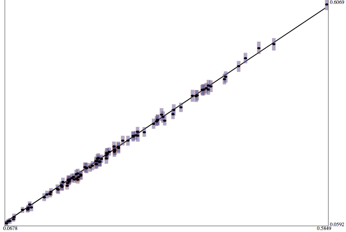
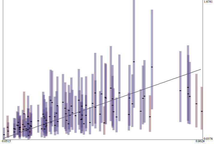
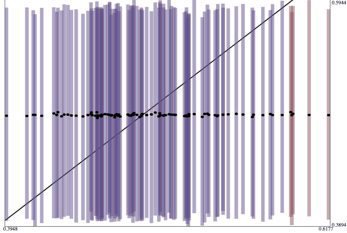
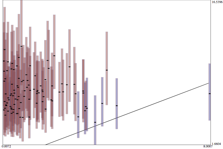
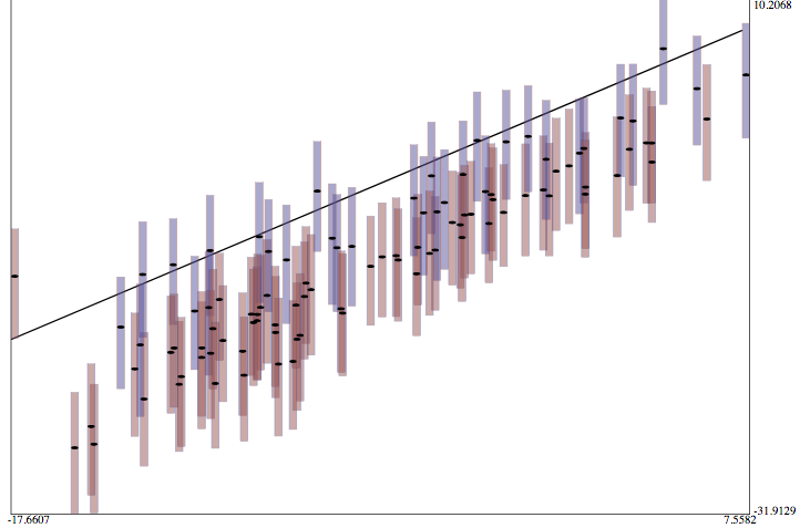
If an output file is specified, CoverageCalcaulator also generates an HTML file with bar graphs (in svg ) showing how well each item in the log file covers the true value, as well as tab separated (tsv) files containing the data, so you can import them in for example R to produce customised graphs. Below some examples with good coverage, and strong, medium and weak ability to learn the parameter, followed by over estimated and under estimated parameters.
Graphs show true value on x-axis and estimates on y-axis. Black line shows where x equals y axis, and where ideally most of the probability mass is concentrated. Black dots are means of estimates. Bars indicate 95% HPDs where blue bars cover the true value and red ones do not. Ideally 95 out of 100 bars should be blue.
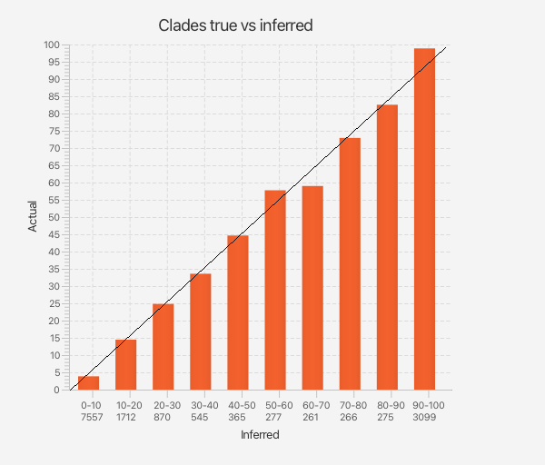
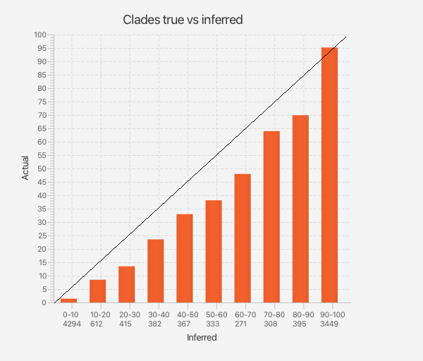
To test whether clade probabilities obtained from the posterior tree distribution are correct, we can create a bar chart showing how often a clade prediction matches the true clade taken from the input trees.
A bar graph is constructed by counting how many inferred probabilities fit in a bin, then calculating how many of the true values are in a certain bin. Each bar represents a 10% sized interval, where the first bar represents predictions in the range 0 to 10%, the second bar ranges from 10% to 20%, etc. The number below the range represents the number of predictions that fit in that range for each of the 100 posterior distributions. For example, there are 3099 predictions in the range 90-100% (last column) in the graph below. The size of the bar is the percentage of times the true prediction is in the bin with the associated prediction.
- If the inferred clade probabilities are correct, the bars should cross the x=y line.
- If they are too high, the bars will be below the x=y line.
- If they are too low, the bars will be above the x=y line.
To create a bar graph, use the CladeCoverageCalculator tool. It has the following options:
- truth (TreeFile): trace file with true infection information (required)
- prefix (File): log file name without the number and '.log' missing. It is assumed there are as many log files as there are entries in the truth file (required)
- out (OutFile): output file, or stdout if not specified (optional, default: [[none]])
- burnin (Integer): percentage of trees to used as burn-in (and will be ignored) (optional, default: 10)
- png (OutFile): name of file to write bar-chart plot (optional, default: [[none]])
- bins (Integer): number of bins=bars to use for the chart (optional, default: 10)
- skip (Integer): number of trees in truth to skip (optional, default: 1)
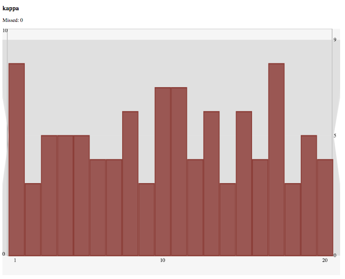
Simulation Based Calibration (SBC) [@talts2018validating] is a way to validate how well true values used to generate data rank inside the inferred distributions. Ranks are binned, and the resulting bins should be uniformly distributed if all is well. Deviation from uniform distributions indicate
- if shaped like a U the posterior is too narrow.
- if shape like inverted U, the posterior is too wide.
- if shaped sloping upwards, the posterior is biased towards lower estimates.
- if shaped sloping downwards, the posterior is biased towards higher estimates.
To run a simulated based calibration study (steps 1-3 as for a coverage study):
- set up XML for desired model and sample from prior
- generate (MCMC) analysis for each of the samples (say 100)
- run the analyses
- use
LogAnalyserto find minimum ESS - run
LogCombinerto sub sample log files and accumulate logs - run
SBCAnalyserto summarise coverage of parameters
A correct implementation is uniformly distributed, like so:
For steps 1-3, see coverage study.
Use LogAnalyser to find minimum ESS -- or run coverage study and minimum ESS will be printed as part of the analysis.
First, we need to determine how much to resample log files. Since samples must be independent for the method to work, we can resample with frequency equal to the chain length divided by minimum ESS.
Run LogCombiner to sub sample log files and accumulate logs. To run from command line, use
/path/to/beast/bin/logcombiner -resample <resample> -log <name>-?.log <name>-??.log <name>-???.log -o combined.log
where <resample> is the resample frequency (= chain length/minium ESS), and <name>- the name of the log file. Note that if you numbered the log files 0,...,9,10,...,99,100,...,999 using <name>-*.log will put entries in an alphabetic order, which is probably not what you want.
SBCAnalyser can be run with the BEAST app launcher, and outputs a report and (if an output directory is specified). It has the following arguments:
SBCAnalyser has the following inputs:
- log
<filename>: log file containing actual values (required) - skip
<integer>: numer of log file lines to skip (optional, default: 1) - logAnalyser
<filename>: file produced by logcombiner, combining the trace log files associated with entries in the 'log' file - bins
<integer>: number of bins to represent prior distribution. If not specified (or not positive) use number of samples from posterior + 1 (L+1 in the paper) (optional, default: -1) - outputDir
<directory>: output directory for SVG bar charts (optional, default: [[none]]) - useRankedBins
<boolean>: if true use ranking wrt prior to find bins. If false, use empirical bins based on prior. (optional, default: true) - exclude
x,y,z: comma separated list of entries to exclude from the analysis. By default,posterior,priorandlikelihoodare excluded.
Note that it compares entries from the prior to posterior, so items like likelihood, posterior, treeLikelihood and clockRate seem very wrong, but that can be ignored, since these were not part of the prior or (for clockRate) we know beforehand the prior differs substantially from the posterior.
99%lo << mean << 99%up = -1 << 5 << 10
                                                	missed	bin0	bin1	bin2	bin3	bin4	bin5	bin6	bin7	bin8	bin9	bin10	bin11	bin12	bin13	bin14	bin15	bin16	bin17	bin18	bin19
posterior                                       	1	0	0	0	0	0	0	0	0	0	0	0	0	0	0	0	0	0	0	0	100
likelihood                                      	1	0	0	0	0	0	0	0	0	0	0	0	0	0	0	0	0	0	0	0	100
prior                                           	0	8	5	6	6	4	3	7	5	1	7	3	9	8	4	3	6	3	6	4	2
treeLikelihood.dna                              	1	0	0	0	0	0	0	0	0	0	0	0	0	0	0	0	0	0	0	0	100
TreeHeight                                      	1	3	5	3	3	2	4	5	3	4	6	7	6	5	3	17	5	6	7	2	4
kappa                                           	0	8	3	5	5	5	4	4	6	3	7	7	4	6	3	6	4	8	3	5	4
gammaShape                                      	0	6	6	2	4	3	2	2	6	6	5	7	6	3	4	4	7	7	6	9	5
popSize                                         	1	1	3	1	3	2	6	1	3	1	5	9	5	4	5	11	10	9	5	10	6
CoalescentConstant                              	0	7	5	0	7	9	5	5	4	5	9	6	3	7	5	7	5	4	5	1	1
parameter.hyperInverseGamma-beta-PopSizePrior   	0	6	3	2	6	3	3	3	7	3	8	10	5	6	6	2	7	2	5	6	7
HyperPrior.hyperInverseGamma-beta-PopSizePrior  	1	11	2	5	4	5	3	5	10	1	10	10	2	8	1	3	6	3	2	5	4
monophyletic(root)                              	1	0	0	0	0	0	0	0	0	0	100	0	0	0	0	0	0	0	0	0	0
logP(mrca(root))                                	0	5	5	1	4	2	4	6	5	4	4	7	5	8	5	6	7	8	4	5	5
mrca.age(root)                                  	1	3	5	3	3	2	4	5	3	4	6	7	6	5	3	17	5	6	7	2	4
clockRate                                       	1	0	0	0	0	0	0	0	0	0	0	0	0	0	0	0	0	0	0	0	100
freqParameter.1                                 	1	4	4	7	3	6	7	4	6	1	6	6	6	2	2	6	4	5	2	5	14
freqParameter.2                                 	0	6	9	3	5	4	7	4	4	1	8	7	8	2	4	6	5	8	2	4	3
freqParameter.3                                 	0	6	4	6	8	8	5	4	5	4	6	4	2	4	8	1	7	7	3	3	5
freqParameter.4                                 	0	9	1	2	5	4	3	4	6	3	2	8	7	4	6	6	7	6	6	7	4
Done!
Currently, you need to build from source (which depends on BEAST 2, BEASTlabs and MASTER code) and install by hand (see "install by hand" section in managing packages.
Quick guide
- clone BEAST 2, BEASTlabs, MASTER, and Experimenter all in same directory.
- build BEAST 2 (using
ant Linuxin the beast2 folder), then BEASTLabs (usingant addonin the BEASTLabs folder), and MASTER (usingantin the MASTER folder) then Experimenter (again, usingant addonin the Experimenter folder) packages. - install BEASTlabs (using the package manager, or via BEAUti's
File/Manage pacakgesmenu). - install Experimenter package by creating
Experimenterfolder in your BEAST package folder, and unzip the fileExperimenter/build/dist/Experimenter.addon.v0.0.1.zip(assuming version 0.0.1).
