PhotFDTD/Pyphot passive, with fdtd and phisol as the underlying codes, realizes 3D time domain simulation of optical transmission and 2D mode computation for optical transmission, along with packaged waveguides and dozens of user-friendly examples.
PhotFDTD/Pyphot passive,以fdtd 和phisol为底层代码,实现了光传输的三维时域仿真和二维模式计算,同时提供了已经封装好的波导和数十个方便使用者的示例。
- Waveguide - 直波导
- Arc - 圆弧
- Sbend - S型波导
- Ysplitter - Y分支波导
- Cone (fiber) - 圆锥光纤
- Ellipsoid fiber - 椭圆形光纤
- (Single mode) fiber - 单模光纤
- Fan-shaped waveguide grating (fwg) - 扇形波导光栅
- Directional coupler - 方向耦合器
- Mmi (Multimode-interferometer) - 多模耦合干涉器
- Ring (resonator) - 环形谐振腔
- Photonic Crystal (PC) - 光子晶体
- Thin film filter (TFF) - 薄膜滤波器
- Mach–Zehnder interferometer (MZI) (in progress) - 马赫曾德干涉仪(未完成)
The development version can be installed by cloning the repository
git clone https://github.com/flaport/fdtd
Install requirements
pip install -r requirements.txt
You can also install it by downloading the .zip file directly and extracting it.
Here is an example of basic_ex.py in folder "./examples" to show the workflow and usage of photfdtd. This example shows a 2D simulation of a basic straight waveguide. 本示例展示了一个基础矩形波导的二维仿真
Import required classes
from photfdtd import Waveguide, Grid, Index
Set material and background index 设置材料与背景折射率
background_index = 1.0
Choose Si as the material of the waveguide, index_Re_Si and index_Im_Si are the real part and imaginary part of refractive index of Si at 1550nm, respectively.
index_Si = Index(material="Si")
index_Re_Si, index_Im_Si = index_Si.get_refractive_index(wavelength=1.55e-6)
Create a 2D (y-z) simulation region of 3um x 8um, with a grid spacing of 20nm. 新建仿真空间
    grid = Grid(grid_xlength=3e-6, grid_ylength=1, grid_zlength=8e-6,
                grid_spacing=20e-9,
                permittivity=background_index ** 2,
                foldername="basic_ex")
Set a waveguide of 200nm x 5um and add it into simulation region (grid):
waveguide = Waveguide(
        xlength=200e-9, ylength=1, zlength=5e-6, refractive_index=index_Re_Si, name="waveguide", grid=grid)
Add the waveguide to the grid, it will automatically be placed at the center of the grid. If the waveguide exceeds the grid region, an error message will be displayed.
grid.add_object(waveguide)
Set a line source with center wavelength at 1550nm, the default profile of source is CW. 设置一个1550nm的CW线光源 The x, y, z parameters specify the center position of the source (same as waveguides and detectors). If they are not set by users, it will be automatically set to the center of the grid region.
grid.set_source(source_type="linesource", wavelength=1550e-9, name="source", x=75, y=0, z=60,
                    xlength=400e-9, ylength=0, zlength=0, polarization="x")
Set a line detector 设置一个线监视器 In general, the detector is necessary for calculating the S-parameters and the Fourier transform, but if simulation data in the time domain are not needed, then this step can be omitted.
grid.set_detector(detector_type="linedetector",
                  name="detector",
                  x=75,
                  y=0,
                  z=300,
                  xlength=400e-9,
                  ylength=0,
                  zlength=0
                  )
Now we can plot the geometry and the index map.
grid.save_fig()
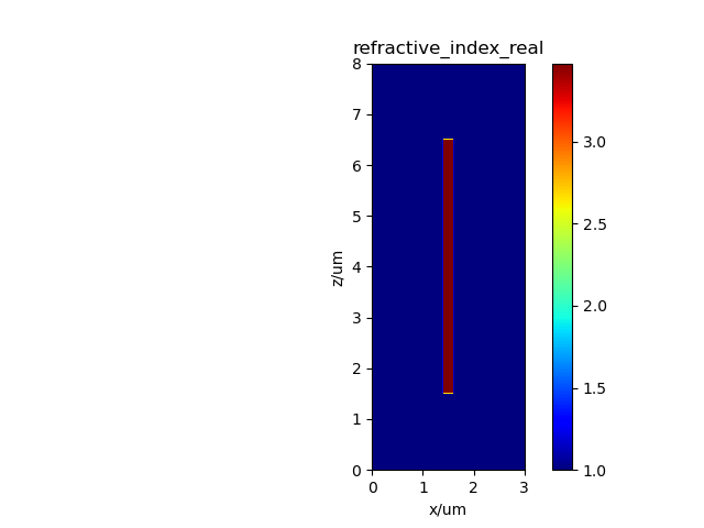
Plot the refractive index map on z=0 绘制z=0截面折射率分布
grid.plot_n()
Run the FDTD simulation 运行仿真
grid.run()
Save result of simulation. The result will be saved in a .npz file, which is a numpy file. It can be read by using grid.read_simulation method, refer to read_FDTD_simulation.py for further details. 保存仿真结果
grid.save_simulation()
# grid = grid.read_simulation(folder=grid.folder)
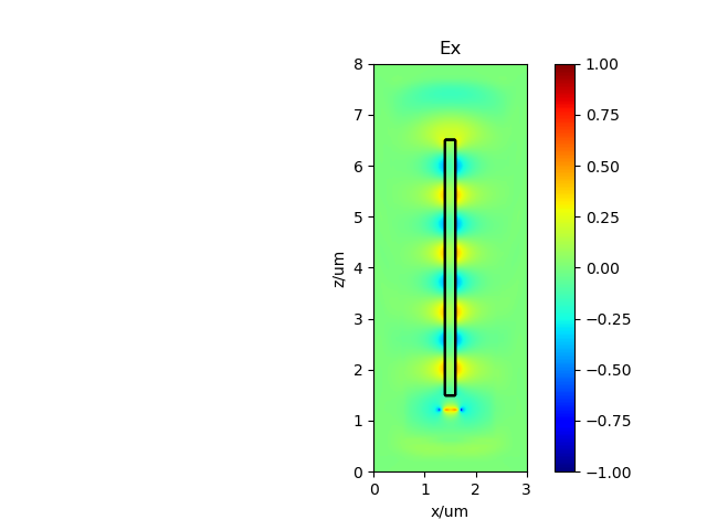
The field distribution at the end of the simulation. 绘制仿真结束时刻空间场分布
Grid.plot_field(grid=grid, field="E", field_axis="x", axis="y", axis_index=0, vmin=-1, vmax=1)
If a detector has been added, the change curve of time domain at a certain point can be plotted, here choose index=30, that is, the center of the detector. 如果添加了监视器,还可以绘制某一点时域场变化曲线,这里选择index=10. 即监视器中心
Grid.plot_fieldtime(folder=grid.folder, grid=grid, field_axis="z", index=10, name_det="detector")
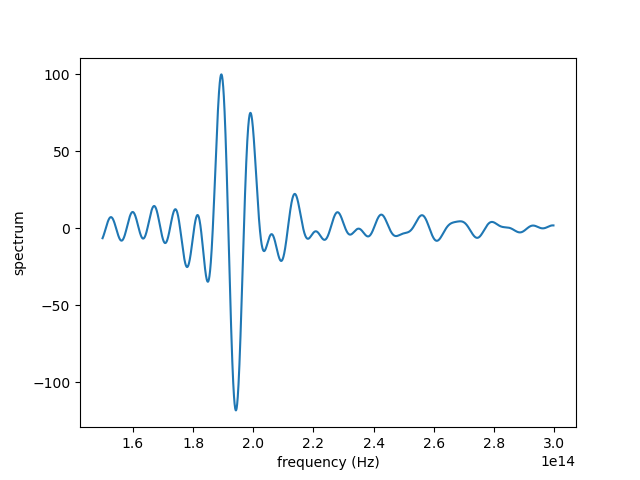
With a detector, we can also draw a frequency spectrum.
Grid.compute_frequency_domain(grid=grid, wl_start=1000e-9, wl_end=2000e-9, name_det="detector",
                                  index=10, field_axis="x", field="E", folder=None)
In the examples directory, you can see examples of various optical devices, e.g. waveguide_ex.py represents an example of a straight waveguide.
Here is an example of solving modes of a single mode fiber from "fiber_ex.py" to analyze a single mode fiber using photfdtd. This example demonstrates the setup and usage of photfdtd mode solver. Parameters of the single mode fiber are as follows:
# Single mode fiber 单模光纤模式分析
# clad refractive index:1.4437 包层折射率
# core refractive index:1.4504 纤芯折射率
# core radius:4um
# Pml thickness:3um
# wavelength:1.55um
Import required classes:
from photfdtd import Fiber, Grid, Solve
Set background index:
background_index = 1.4437
Create simulation region (grid) 新建一个 grid 对象
grid = Grid(grid_xlength=200 * 200e-9, grid_ylength=200 * 200e-9, grid_zlength=1, grid_spacing=200e-9,
            foldername="test_fiber", permittivity=background_index ** 2)
Set fiber parameters and add it to grid
fiber = Fiber(length=1 * 200e-9, radius=[20 * 200e-9, 40 * 200e-9], refractive_index=[1.4504, 1.4555], name='fiber', axis='z', grid=grid)
grid.add_object(fiber)
Create a Solve variant, which is essential for solving mode 创建solve类变量
solve = Solve(grid=grid,
              axis="z",
              filepath=grid.folder,
              index=0
              )
Refractive index plot and geometry plot 绘制折射率分布
solve.plot()
# We can plot the geometry now
绘制x=0截面结构图
grid.save_fig(axis="z", axis_number=0)
Caculate 2 modes around 1.4504 at 1.55um, the boundaries are PML 计算这个截面处,波长1.55um,折射率1.4504附近的2个模式,边界条件选择在四个方向上都是pml
data = solve.calculate_mode(lam=1550e-9, neff=1.4504, neigs=20,
                            x_boundary_low="pml", y_boundary_low="pml",
                            x_boundary_high="pml",
                            y_boundary_high="pml",
                            background_index=background_index)
Save results
Solve.save_mode(solve.filepath, data)
Draw results
Solve.draw_mode(filepath=solve.filepath, data=data, content="amplitude")
# Solve.draw_mode(filepath=solve.filepath, data=data, content="real_part")
# Solve.draw_mode(filepath=solve.filepath, data=data, content="imaginary_part")
# Solve.draw_mode(filepath=solve.filepath, data=data, content="phase")
开发者文档 提供了对于开发者的指导。


