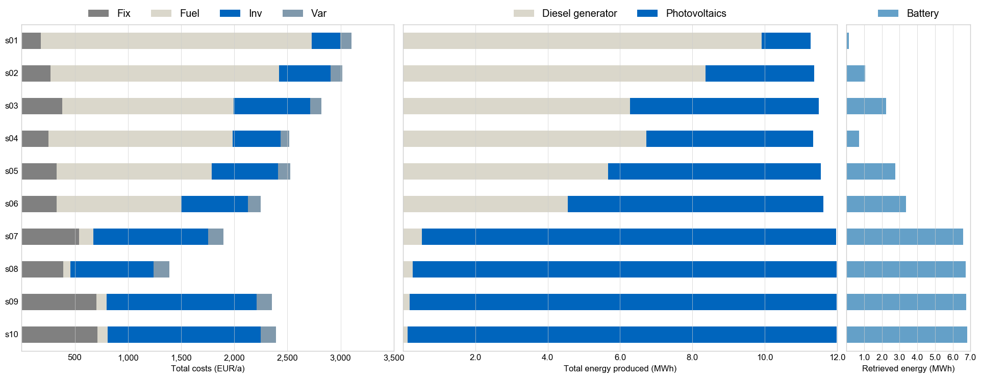
This branch contains a small example study with one site, custom run and comparison script and even dares to slightly modify the urbs.plot function to automatically skip the empty plots for demand side management (DSM). It also demonstrates how to write a custom scenario generator function, a feat that is enabled by Python's capability to hand functions around just like ordinary objects.

As this version of the model is outdated (state early 2017), it can be run with its main dependencies pinned to the same point in time. To install the dependencies as specified in file environment.yml, you can use the following steps:

conda env create -f environment.yml
conda activate urbs-2017

To verify that the environment is active, either run the above within Anaconda Prompt, which displays the active environment to the left of your prompt:

# Windows
(urbs-2017) C:\Users\ojdo\src\urbs>
# Linux
(urbs-2017) /home/ojdo/src/urbs$

or instead run command conda env list, which marks the active environment with an asterisk (*):

# conda environments:
base                     C:\ProgramData\Anaconda3
urbs-2017             *  C:\Users\ojdo\.conda\envs\urbs-2017

File run1node.py is the main entry point, which contains user settings like solver and how many timesteps (some days for debugging, weeks or a whole year for the actual study) should be included in the optimization. Results (spreadsheets and timeseries plots) are generated within a timestamped subdirectory within result.

File comp.py can be run after a successful optimization run to generate a condensed cross-scenario comparison spreadsheet + plot. It automatically analyses the newest subfolder within result, or a target directory can be specified.

Both files are meant as a demonstration and basis for one's own optimization and analyses scripts.