![]()
Easily generate graphs using recorded data from your chronograph. Supports LabRadar and MagnetoSpeed with SD card. Create customizable graphs and charts comparing charge weight and velocity without manually entering your chronograph data. Additionally supports creating graphs for seating depth testing.
Table of contents:
- Quick Start
- Round-Robin (OCW) and Satterlee Testing
- Seating Depth Testing
- Building ChronoPlotter from Source
First, download and run ChronoPlotter for your operating system:
- Windows: ChronoPlotter.exe download
- MacOS: ChronoPlotter.dmg download
If your system is not listed above, check out the Building ChronoPlotter from Source section.
The program's main screen will show:

Make sure the SD card from your LabRadar or MagnetoSpeed is plugged into your computer.
- For LabRadar: Click the
Select LabRadar directorybutton, navigate to your SD card, and clickSelect Folderto confirm. - For MagnetoSpeed: Click the
Select MangetoSpeed filebutton, navigate to your SD card, and select theLOG.CSVfile.
The following example shows a LabRadar SD card:

The program should now be populated with all of your recorded data:
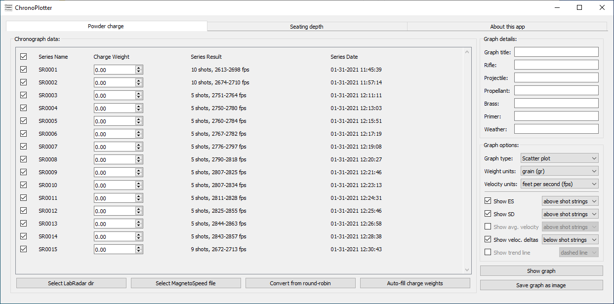
Uncheck any series you don't want to include in the graph. Then enter a charge weight for each series, or click the Auto-fill charge weights button to automate the process:

To include details in the graph about the components used in testing, additionally fill in the text fields on the right:

Clicking Show graph pops open a new window with a preview of the generated graph. Note: This does not save your graph, only displays it.
The graph will look something like this:

You can alternatively create a line chart with standard deviation error bars by selecting it from the Graph type drop-down.

By default, ChronoPlotter displays ES (Extreme Spread), SD (Standard Deviation), and the series-to-series difference in velocity for each series in the graph. The average (mean) velocity for each series can also be displayed but is unchecked by default. You can add, remove, or change the location of these details in the graph under the Graph options section.
Close the preview window, making sure not to close ChronoPlotter itself. Finally, click Save graph as image to save your graph as a .PNG, .JPG, or .PDF file.
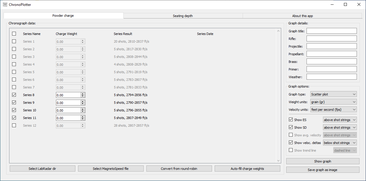
ChronoPlotter supports chronograph data recorded using the "round-robin" method popular with OCW testing. First, uncheck any series not part of the round-robin:
Click Convert from round-robin to open this dialog:

Then click OK to convert the series data into traditional series suitable for graphing. Note that ChronoPlotter does not alter your CSV files, this only converts the data loaded in the program:

Likewise, this same feature can be used to convert data recorded using the Satterlee method. This is because at its core Satterlee is simply a "one shot round-robin" test. To do so, uncheck all other series except for the one series containing Satterlee data, then click Convert from round-robin and proceed as usual.
Thanks to TallMikeSTL for contributing test data.
In addition to powder charge graphs, ChronoPlotter also supports creating graphs comparing bullet seating depth and group size. This data must be separately recorded and inputted by the shooter.
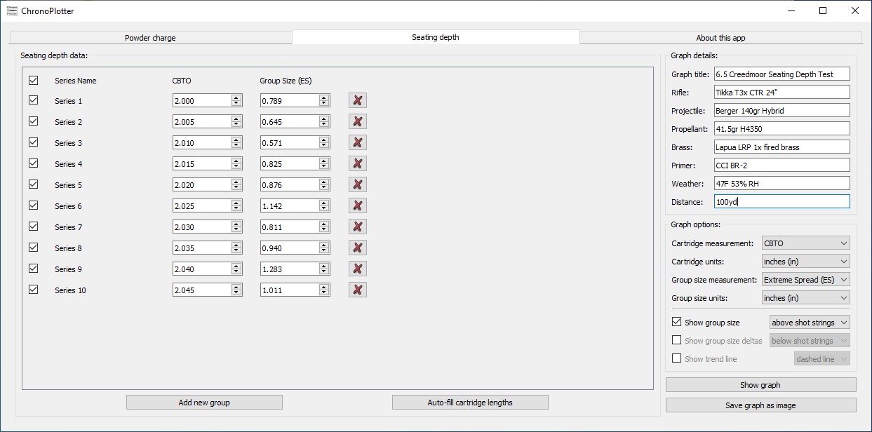
Begin by clicking the Seating depth tab at top:

By default, a single empty series is created. Click the Add new group button to create additional series for each cartridge length being tested. Then enter a cartridge length for each series, or click the Auto-fill cartridge lengths button to automate the process:

Then proceed to enter the group size for each series. NOTE: ChronoPlotter defaults to CBTO (Cartridge Base to Ogive) for cartridge length and ES (Extreme Spread) for group size measurements. Other measurements may instead be selected under the Graph options section on the right, if desired.
To include details in the graph about the components used in testing, additionally fill in the text fields on the right:
Clicking Show graph pops open a new window with a preview of the generated graph. Note: This does not save your graph, only displays it.
The graph will look something like this:

By default, ChronoPlotter displays the group size for each series in the graph. The series-to-series difference in group size can also be displayed but is unchecked by default. You can add, remove, or change the location of these details in the graph under the Graph options section.
Close the preview window, making sure not to close ChronoPlotter itself. Finally, click Save graph as image to save your graph as a .PNG, .JPG, or .PDF file.
For most general purposes, use the prebuilt executable files available for download at the top of the quick start section.
If your operating system is not listed, or if you'd like to make changes to the program, ChronoPlotter can alternatively be built from source. The project is written using the Qt framework. It targets Qt version 5.12.2, but other Qt versions may potentially work as well.
To build for Ubuntu, first install dependencies:
$ sudo apt-get install build-essential qt5-default qt5-qmake
Then build with:
$ qmake
$ make
The binary ChronoPlotter will then be created. Other Linux distributions may require different dependencies but will follow a similar process.
To build for MacOS, first install dependencies:
$ brew install qt5
$ brew link qt5 --force
Then build with:
$ qmake
$ make
The app directory ChronoPlotter.app/ will then be created.
To build for Windows, first install Qt then run the following commands:
> qmake -config release
> mingw32-make
The binary release\ChronoPlotter.exe will then be created.
At this time, only MingGW has been tested for building on Windows. It may be possible to use MSVC.