Easily generate graphs using recorded data from your chronograph. Supports LabRadar and MagnetoSpeed with SD card. Create customizable graphs and charts comparing charge weight and velocity without manually entering your chronograph data.

Table of contents:

• Quick Start
• Round-Robin (OCW) and Satterlee Testing
• Running ChronoPlotter with Python
• Notes About PyInstaller

If you're looking to quickly get started with ChronoPlotter, download and run the prebuilt program:

• Windows: ChronoPlotter.exe download
• MacOS: ChronoPlotter.dmg download

Nerds and power users should reference the Running ChronoPlotter with Python section.

Note: The program may take a few moments to start. The program's main screen will then show:

Make sure the SD card from your LabRadar or MagnetoSpeed is plugged into your computer. Then click Select directory, navigate to your SD card, and click Select Folder to confirm. The following example shows a LabRadar SD card:

The program should now be populated with all of your recorded data:

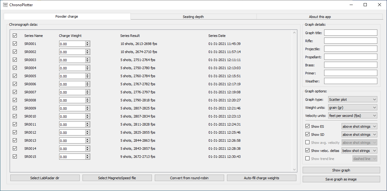
Uncheck any series you don't want to include in the graph. Then enter a charge weight for each series, or click the Auto-fill charge weights button to automate the process:

To include details in the graph about the components used in testing, additionally fill in the text fields on the right:

Clicking Show graph pops open a new window with a preview of the generated graph. Note: This does not save your graph, only displays it.

The graph will look something like this:

You can alternatively create a line chart with standard deviation error bars by selecting it from the Graph type drop-down.

By default, ChronoPlotter includes ES (Extreme Spread), SD (Standard Deviation), and the series-to-series difference in velocity for each series in the graph. The average (mean) velocity for each series can also be included but is unchecked by default. You can add, remove, or change the location of these details in the graph under the Graph options section.

Close the preview window, making sure not to close ChronoPlotter itself. Finally, click Save graph as image to save your graph as a .PNG, .SVG, or .PDF file.

ChronoPlotter supports chronograph data recorded using the "round-robin" method popular with OCW testing. First, uncheck any series not part of the round-robin:

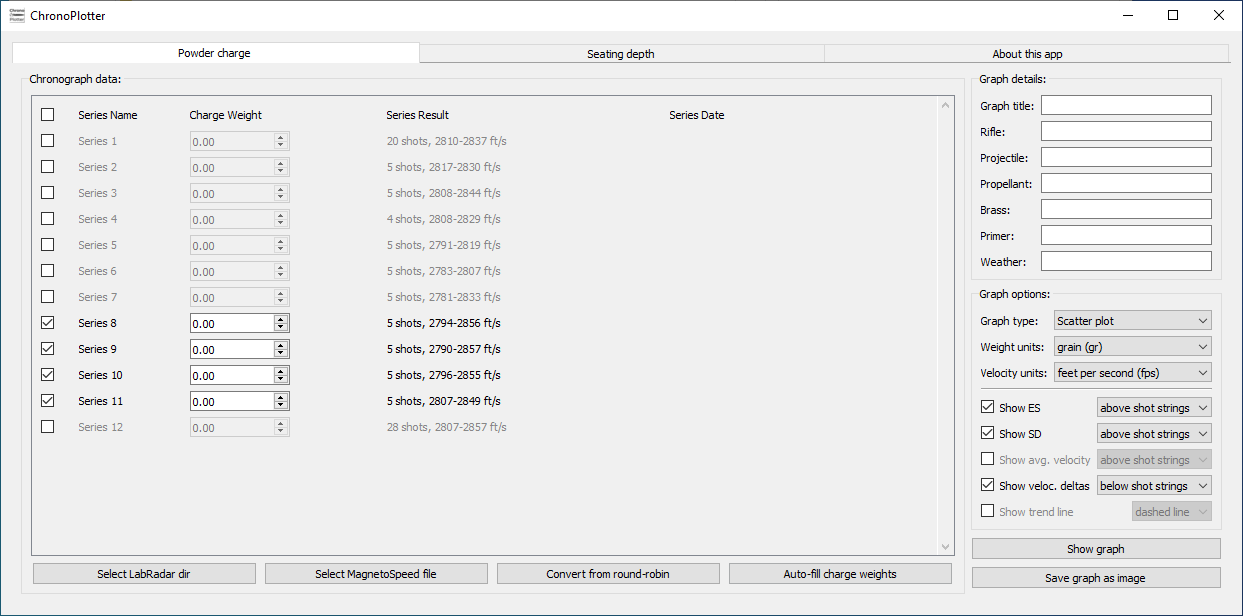
Click Convert from round-robin to open this dialog:

Then click OK to convert the series data into traditional series suitable for graphing. Note that ChronoPlotter does not alter your CSV files, this only converts the data loaded in the program:

Likewise, this same feature can be used to convert data recorded using the Satterlee method. This is because at its core Satterlee is simply a "one shot round-robin" test. To do so, uncheck all other series except for the one series containing Satterlee data, then click Convert from round-robin and proceed as usual.

Thanks to TallMikeSTL for contributing test data.

Users can directly run ChronoPlotter.py as a Python script instead of using the prebuilt binaries. Python 3.5+ is required (for PyQt5)

Install the following dependencies:

pip3 install --upgrade pip
pip3 install numpy matplotlib PyQt5

Then run:

python3 ChronoPlotter.py

ChronoPlotter uses PyInstaller to generate single file executables for ease of distribution. It does not come without certain trade-offs, though. PyInstaller works by bundling an entire base Python installation + additional modules in a single file, and unpacking it to a temporary directory every time the executable is run. This results in large executables and slow program start time (up to 15 seconds on slow disks!)

A lot of time has been spent trying to optimize the ChronoPlotter executables. PyInstaller was chosen for its multi-platform support, ability to create single file executables, and current support by project maintainers. It also features a "hooks" subsystem that optimizes out unused portions of common Python modules. Other Python "freezing" solutions such as py2exe and cx_Freeze, as well as Python compilers such as Nuitka, were also explored but either ran into errors or produced even larger files than PyInstaller.

Focus was instead placed on optimizing the PyInstaller-created executables themselves. ChronoPlotter uses matplotlib and PyQt5 which are both notoriously massive, complex dependencies that are difficult to efficiently freeze. By default, PyInstaller bundles all matplotlib backend modules it can find, however modifying PyInstaller to include a hardcoded whitelist provided only marginal improvement. Configuring PyInstaller to pack files with UPX provided the greatest file size savings (almost 10mb smaller) but increased the executable start time by upwards of 20-40% which became unacceptable on slow disks.

At the end of the day, ChronoPlotter ships standard PyInstaller single file executables. The correct solution is to rewrite the entire project in C++ and swap out matplotlib for a different native graphing solution. That's going to be a whole thing though, and there's something nice about the versatility and human-readability of Python. If you have any suggestions to improve ChronoPlotter or the way it's distributed, feel free to open an issue on the tracker.