A bike-sharing prediction service is a useful tool to plan daily supply of bikes. The main goal is to create an end to end service with the main characteristics required in a production environment: possibility of monitoring in production with possible consequent refinement of the prediction model, reproducibility of the entire workflow, quality checks and automation.

The problem is assisting a bike-sharing activity in taking decisions about the supply of bikes over time, to promptly react to demand fluctuations. The specific objective is to predict the hourly count of rented bikes.

For this project, the predictions are based on historical data from the bike-sharing system of the city of Seoul, in South Korea. Ddareungi (Seoul Bike) is Seoul, South Korea’s bike-sharing system. Ddareungi started as a leisure activity but has transformed into a popular means of transportation. There is a dataset originally extracted from the official Seoul Open Data Plaza and that was already used in scientific research activities (see references). It is publicly available in the UCI machine learning Repository:

Seoul Bike Sharing Demand. (2020). UCI Machine Learning Repository. https://doi.org/10.24432/C5F62R.

It is a tabular dataset, comprising 8760 rows and 14 columns. Here below the name and short explanation of each column (variable):

• Date : year-month-day
• Rented Bike count : Count of bikes rented at each hour
• Hour : Hour of he day
• Temperature : Temperature in Celsius
• Humidity : %
• Windspeed : m/s
• Visibility : 10m
• Dew point temperature : Temperature in Celsius
• Solar radiation : MJ/m2
• Rainfall : mm
• Snowfall : cm
• Seasons : Winter, Spring, Summer, Autumn
• Holiday : Holiday/No holiday
• Functional Day : NoFunc(Non Functional Hours), Fun(Functional hours)

The data stored in a row are values for a fixed hour of the day. The dataset spans from December, 1, 2017 to November, 30, 2018. The Rented Bike count is the target variable in this problem. This will be treated as a regression problem.

• Sathishkumar V E & Yongyun Cho (2020). A rule-based model for Seoul Bike sharing demand prediction using weather data, European Journal of Remote Sensing, DOI:10.1080/22797254.2020.1725789
• Ngo, T.T., Pham, H.T., Acosta, J.G., & Derrible, S. (2022). Predicting Bike-Sharing Demand Using Random Forest. Journal of Science and Transport Technology.

The whole development has been done in an isolated virtual environment. I have chosen Poetry as Python dependency manager. For better reproducibility, all the employed libraries are recorded with pinned versions. Among the best coding practices adopted are the usage of linters, formatters and pre-commit hooks

The whole data preparation, the Exploratory Data Analysis and the definition of a baseline model are done inside the bike_count.ipynb notebook. I have held out part of the dataset in order to simulate a monitoring task during the deployment in production. In particular, from the total 8760 samples, I have stored 6576 samples from Winter, Spring and Summer in ref_data.csv and the remaining 2184 samples (Autumn) have been stored in curr_data.csv.

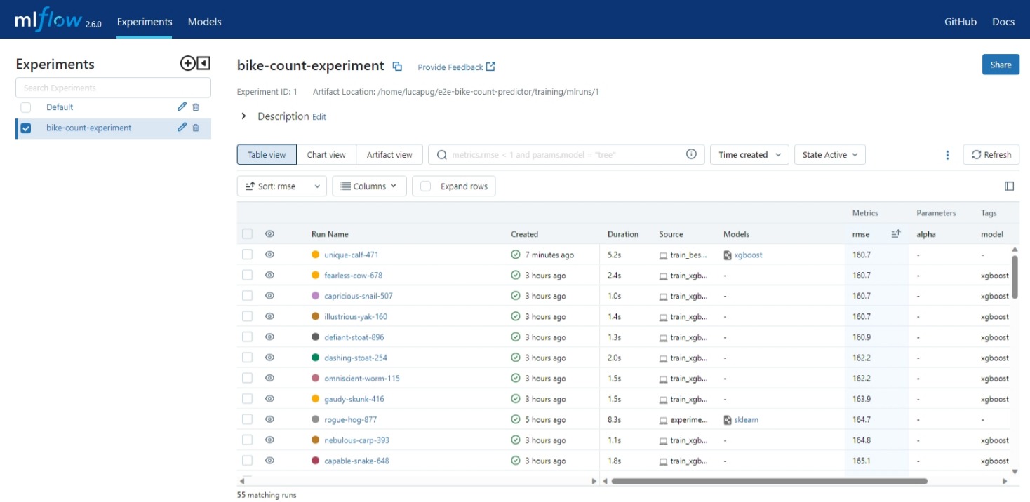
All the experiments are contained in the training folder and they are tracked using MLFlow. experiments.py is a script obtained from a refactored version of the bike_count notebook. It containes runs of the mlflow experiment named 'bike-count-experiment'. While train_xbg.py contains runs of the same mlflow experiment, created by fine tuning the xgb model with the aid of the hyperopt library. In the end, the xgboost model with the best parameters is chosen as best model due to its performance in terms of rmse and model file dimension.

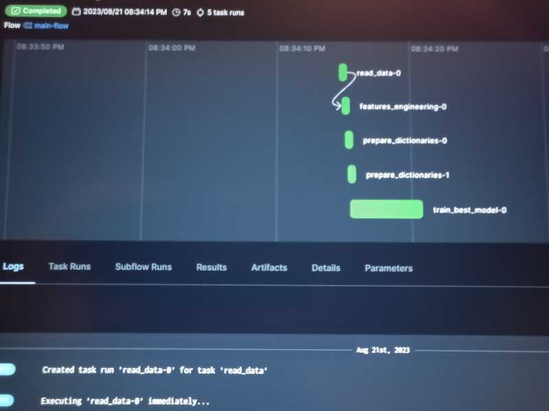
For the choiced best_model a script was created, named train_best_flow.py, where the training pipeline for the model with the best params is executed as flow orchestrated by Prefect. Once executed, here below is a screenshot of the Prefect dashboard.

As a second product of the script, the pipeline parameters are registered in the mlflow dashboard as a new run of the bike-count-experiment

In predict.py a Flask app is defined to make inferences, adopting the preprocessor and the model corresponding to the the best_params run of the 'bike-count-experiment'. By launching a gunicorn server (gunicorn --bind=0.0.0.0:9696 predict:app), the inference app becomes ready to receive requests. One of these requests is contained in test.py. If this file is executed, the inference result correponding to the input record can be obtained. Now that we have tested the correct functioning of the Flask inference app, we can dockerize the deployment service, in order to make it easily reproducible by others. So the corresponding Dockerfile is created, and from it the Docker image can be built (docker build -t bike-count-prediction-service:v1 .), then a container based on the image can be run (docker run -it --rm -p 9696:9696 bike-count-prediction-service:v1), to verify that we obtain the same result from the execution of test.py

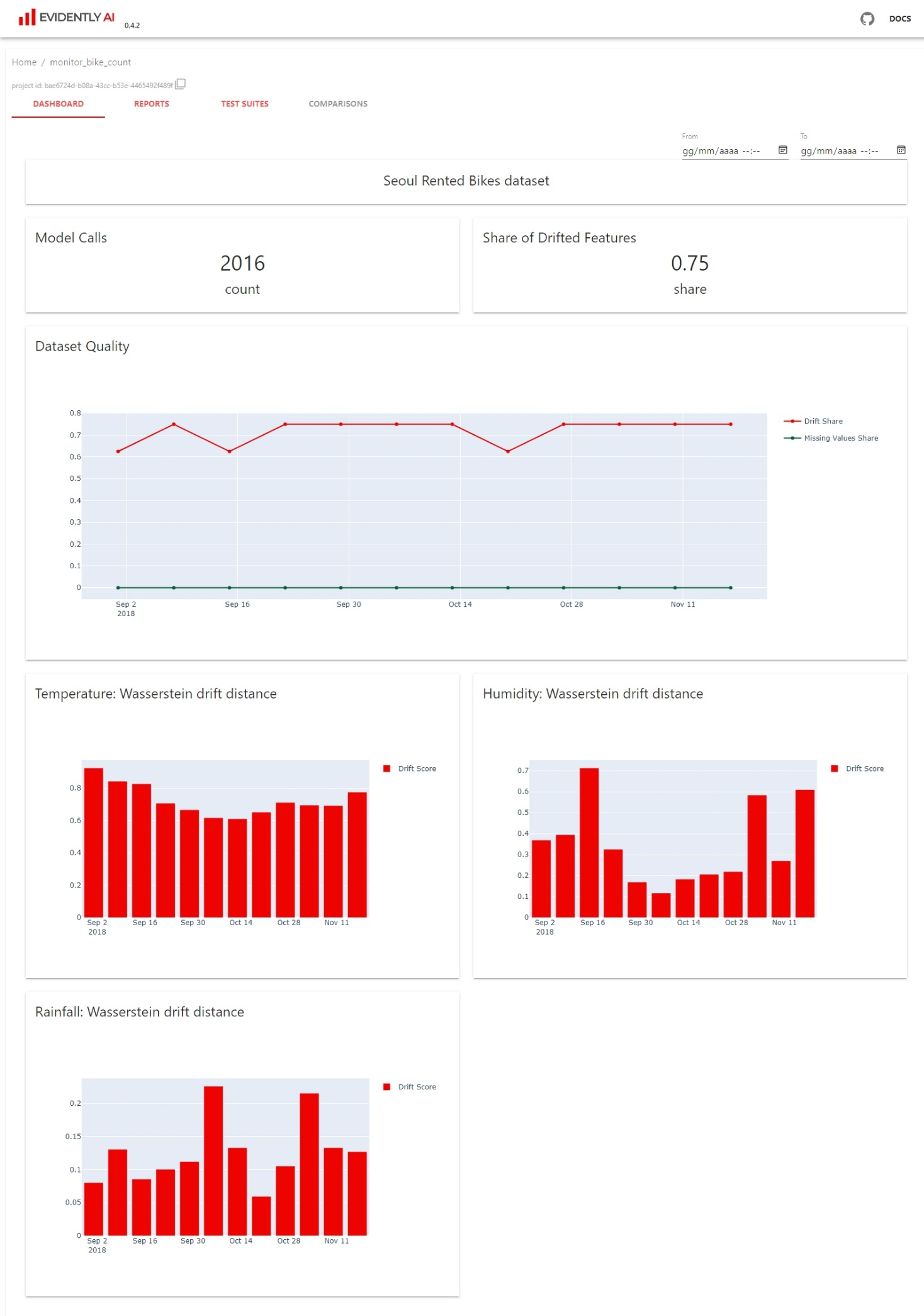
In order to monitor data drift in production, a monitoring component has been created, taking advantage of the Evidently library functionalities. In particular, to simluate production monitoring, from the beginning I have held out part of the dataset to be used as current data. Intentionally, the original dataset split has been done by the Seasons column values, storing in ref_data the records from Winter, Spring and Summer, and the remaining Autumn data is stored as curr_data. Making this choice, there is a high probability of revealing data and column drift. Two kinds of monitoring tasks has been done. A first data drift analysis has been executed in the check_data_drift.ipynb notebook. Here I make use of the whole curr_data in one shot. All the 14 original features are employed in this task (interim data). The second task is more realistic in a production environment and it is more suitable for automation. It is contained in weekly_monitor.py in the monitoring folder. I simulated a weekly monitoring on the 13 weeks of the Autumn season. Taking advantage of the monitoring dashboard, a new feature available from v0.4.0 of Evidently, I launched the dashboard (command: evidently ui), that takes its source of infromation from the snapshots created inside the workspace folder when weekly_monitor.py has been executed. Here below a screencapture from the dashboard.