Climate change is the long-term changes in temperature and weather patterns. Although these changes are natural, since the 1800s, human activities have been the primary driver of climate change owing to the burning of fossil fuels (such as coal, oil, and gas), which produces greenhouse gases. Climate change will impact the lives of future generations. Hence, Climate change is one of the most important concepts in the current scenarios that people need to be aware of. But some people think that climate change is just a hoax or a conspiracy theory while some people think that climate change is a severe threat to life on earth.

In this project, we propose to analyze the opinion of people by performing sentiment analysis on tweets by Twitter users on the topic of Climate Change. We plan to do an exploratory data analysis and train models based on various traditional machine learning algorithms and a Deep Learning Model using Recurrent Neural Network approach using Text in Tweets and the frequency of some keywords as features. By performing this analysis, we get a rough idea of how aware and how supportive people are of the cause of the prevention of climate change and plans can be made to bring awareness to people. We also test our model on unseen data of tweets that we scrapped from Twitter.

By performing this analysis, we get a rough idea of how aware and how supportive people are towards the cause of the prevention of climate change and plans can be made to bring awareness to people.

• Prerequisites
  • Environment
  • Technologies Used
  • Dataset Description
• Model Implementation
  • Data Preprocessing
  • Exploratory Data Analysis
    • Itertools & NLTK Frequent Distance
    • Plotting Most Frequent Words using WordCloud
    • VADER Sentiment Analysis
  • Traditional Machine Learning Approacehs
    • Preparing Data
    • Logistic Regression
    • K Nearest Neighbors
    • Naive Bayes Classifier
    • Random Forest Classifier
  • Deep Learning Approach – LSTM CNN Model
    • Preparing Data
    • Long Short Term Memory Network
  • Results
    • Exploratory Data Analysis
    • VADER
    • Traditional Machine Learning Approacehs
    • Deep Learning Approach – LSTM CNN Model
• Developers
• Links
• References

1. Python 3 Environment (Ancaonda preferred)
2. Python modules required:NumPy,Pandas, Imblearn, Scikit-learn, Keras, Warnings, Copy, Re, Nltk, Itertools, Wordcloud, Opencv2,Matplotlib, Seaborn
3. Web Browser

OR

• Any Python3 IDE installed with above modules.

1. Anaconda Jupyter Notebook

We are using Twitter Climate Change Sentiment Dataset[1] taken from the Kaggle website containing more than 43 thousand tweets based on the topic of climate change in the period between April 27th, 2015, and February 21st, 2018. These tweets are labeled by three reviewers independently into 4 classes:

• 2(News): the tweet links to factual news about climate change
• 1(Pro): the tweet supports the belief of man-made climate change
• 0(Neutral): the tweet neither supports nor refutes the belief in man-made climate change
• -1(Anti): the tweet does not believe in man-made climate change

Data Preprocessing

• We observed that there is a clear class imbalance in the dataset, therefore we performed Random Oversampling to balance the data. To perform the Random oversampling, we used methods defined in the ‘imblearn’ library. The ‘RandomOverSampler’ method of imblearn duplicates minority class data points and balances the majority/minority class ratio. And for our current problem, we do not need texts from the “News (2)” class. Hence, we remove data belonging to class

Exploratory Data Analysis

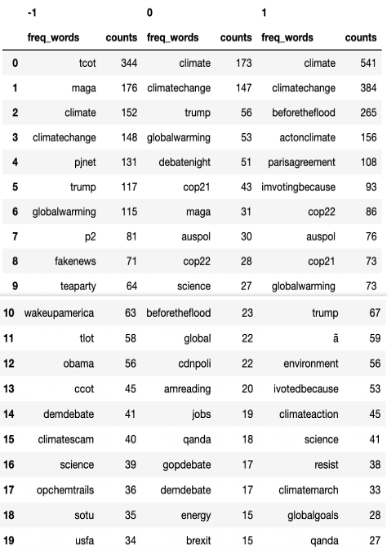
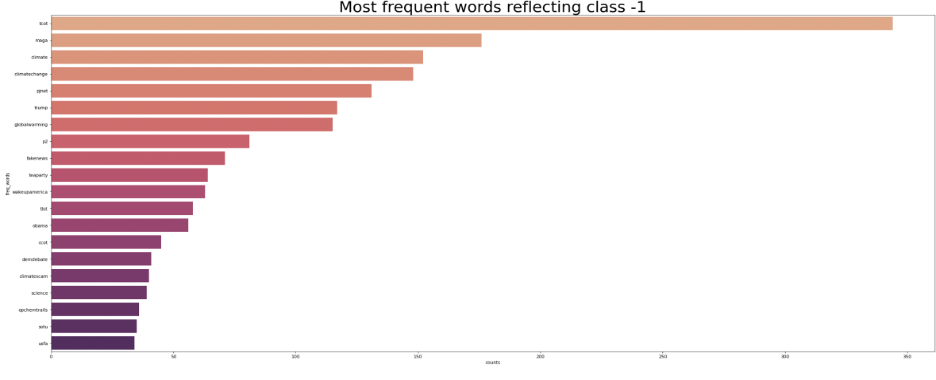
• We find the most frequent words occurring in the tweets of each sentiment. We use Itertools by making a sequence of words occurring in each sentiment class. Then we calculate the frequency of these words occurring in the class set by calculating the rate of recurrence of these words in this entire set by using the FreqDist method from the nltk library. Then we print the frequency of each word in the set and pull the top ten words as the most frequent words in each sentiment.

• We made use of WordCloud for keyword/buzzword analysis i.e., for finding the most used words in the given context of the tweet. WordCloud is one of the easiest ways to show which word mainly(frequently) appears in the set of sentences. WordCloud conveys importance through opacity, so the more translucent a word, the less frequently it appears. Using WordCloud we found keywords/buzzwords in all three contexts (positive, negative, and neutral sentiments).

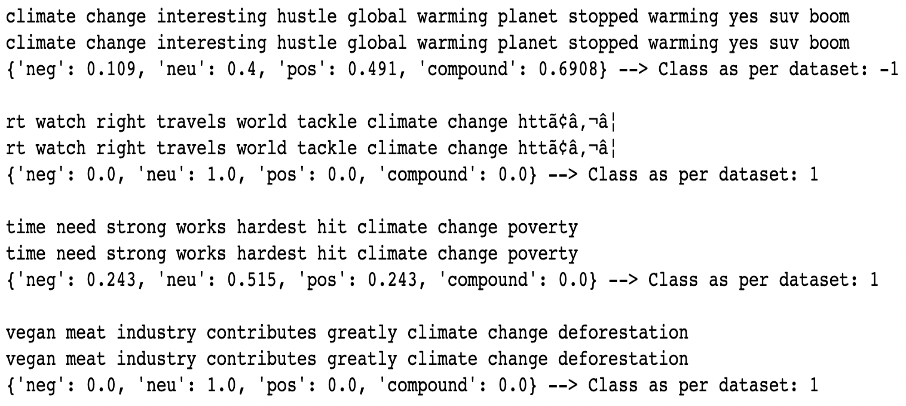
• VADER (Valence Aware Dictionary and sEntiment Reasoner) is a lexicon and rule-based sentiment analysis tool that is specifically attuned to sentiments expressed in social media. Vader has a dictionary of words that maps lexical features to emotion intensities called sentiment scores. And finally depending on the sentiment score of the text, it classifies the text as positive, negative, or neutral. The emotional intensity of an individual word is measured from -4 to 4, where -4 is the most negative sentiment and +4 is the most positive sentiment. The total sentiment score of the entire text is between -1 and 1. If the total sentiment score of the text is more than 0.05 then it is considered positive sentiment. If the total score is less than -0.05 then it is considered negative sentiment otherwise it is classified as neutral sentiment.

Traditional Machine Learning Approaches

• The Tweets dataset is split into train and test datasets with 80-20 random splitting. For applying any machine learning algorithm, the data needs to be readable and statistically analytical formal. For that, we use the TFID Vectorizing method. The role of TFIDFVectorizer is to assign word frequency scores and these scores determine how much the word is contributing to the sentiment. TFIDFVectorizer calculates scores combining 2 concepts, Term Frequency (TF) and Document Frequency (DF). The number of times a phrase appears in a document is known as its Term Frequency. The importance of a phrase in a text is determined by its Term Frequency. The number of documents that include a certain word is known as document frequency. The frequency of a phrase in a document reflects how common it is. These scores are used to train the models.

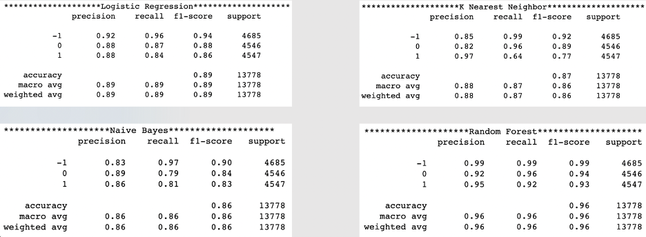
• First, we trained using the Multinomial Logistic Regression Algorithm. Multinomial Logistic Regression is a Logistic Regression generalization that can handle several classes. When the classes are separated linearly, Logistic Regression works well. it's very sensitive to the class balance. We train the model using the sklearn LogisticRegression method. We set the “class_weight” property to “balanced” which is “none” by default. The balanced mode automatically adjusts weights that are inversely proportional to class frequencies in input data. We also set the number of iterations to 1000. The default number of iterations is 100 in the sklearn method, which we modified to 1000.

• Next, we train using the K-Nearest Neighbor algorithm. KNN predicts the values of new data points based on "feature similarity." It computes the similarity between the K closest points of the given data point. We make use of the KNeighborsClassifier method of sklearn to train the model. First, we trained multiple models with different values of K and then decided that the best possible outcome is when k=15. Here we set the weights property to distance i.e., closer neighbors to the point will have more influence than the neighbors which are far away. We make use of Euclidean distance to calculate the distance between 2 points.

• The third Algorithm we used for training is Naïve Bayes. Bayes Theorem is used by Naive Bayes to produce classifications. This is based on the assumption that independent variables are statistically independent. We make use of the MultinomialNB method of sklearn. We have total of three classification methods in Naïve Bayes, Gaussian, Bernoulli, and Multinomial classifications. We made use of Multinomial because it is best for discrete counts, in our case we don’t look if the word is present in the document or not, but we find the frequency of the word in the document. Later, we also tried Complement Naïve Bayes to correct the assumptions of imbalanced classes made by Multinomial Naïve Bayes, but there was not much difference between them both, so we stuck with Multinomial Naïve Bayes.

• Finally, we trained using Random Forest. Random Forests are a tree-based Machine Learning technique that takes advantage of the combined strength of numerous Decision Trees. If-elif-else control flow is similar to that of decision trees, except the measure for each decision boundary is information gain/Gini Index. In Random Forest, you construct a Forest by "planting" a group of Decision Trees together. We made use of the RandomForestClassifier method of sklearn. First, we trained different models of Random Forest using different criteria for calculating maximum features and measuring for decision boundaries. We observed that the Gini Index measure for decision and log2 measure for max features are giving the best possible results, so we finalized those properties.

Deep Learning Approach – LSTM CNN Model

• We used the Tokenizer method to tokenize the message text into a set of tokens. Then we transform this text into a sequence of integers. Then we pad the texts into a set of numbers of equal length using pad_sequence methods defined in the sequence preprocessing library of Keras. In addition to this, we convert the label row of the data frame which defines the class of the tweet into indicator variables. We use this tokenized text as features and indicator variables as target columns for training the LSTM CNN model. And we then split the dataset into three sets – training, validation, and testing sets for training and testing the model.

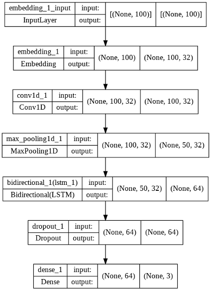
• Long Short-Term Memory Networks are a type of recurrent neural network that excels at tasks with long time delays or has a lot of features to deal with. Because the LSTM has three gates, it can evaluate whether or not the flow should be remembered. The "input gate" determines whether fresh information may be memorized once it is input. The "forget gate" controls how long a value can be stored in memory. The "output gate" regulates how much the value stored in memory influences the block's output activation. As input to the LSTM layer, every tweet is represented as a word embedding matrix. Because of its ability to remember, the LTSM layer can learn previous data, and the new output generated by the LSTM layer is sent into the CNN layer, which can and is good at capturing local features. The output is then passed into the max-pooling and completely connected layers, where it is eventually classified as positive or negative. The network architecture of the model we trained is as follows:

• We train a Bidirectional CNN network using a Keras Sequential Model. We initiate training of the model for a maximum of 20 epochs and we define an Early Stopping condition by monitoring validation loss. We compile the model using the ‘adam’ optimizer and using a loss function of ‘categorical_crossentropy’. We fit and train the model by plotting various evaluation metrics like accuracy, precision, and recall.

Results

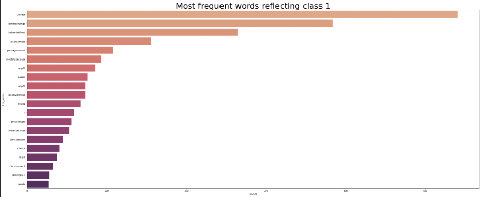
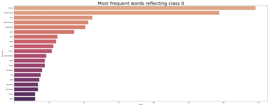
• We have analyzed the tweets using NLTK itertools for the most frequent words in each sentiment and found the following results. The below bar plots show the frequency of the top 20 words in each sentiment.

• We have analyzed the VADER Polarity scores of the tweets in the dataset and the results are not satisfactory and most of the tweets are being given inaccurate scores.

• We have analyzed the VADER Polarity scores of the tweets in the dataset and the results are not satisfactory and most of the tweets are being given inaccurate scores.

• We have trained an LSTM CNN model on the training dataset by concurrently evaluating the model using a validation dataset for 10 epochs. Then we applied the model to unseen test data to predict the classes and calculated the accuracy of the model by plotting the confusion matrix and classification report.

• Kamal Yeshodhar Shastry Gattu
• Venkata Sriram Rachapoodi

GitHub: G K Y SHASTRY

Contact me: [email protected] , [email protected]

Climate Change Twitter Dataset