Scope:
- Camera Calibration
- Distortion Correction
- Perspective Transform
- Color and Gradient Threshold
- Detect Lane Lines
- Determine Lane Curvature
- Impose Lane Boundaries on Original Image
- Output Visual Display of Lane Boundaries and Numerical Estimation of Lane Curvature and Vehicle Position
The first step in the project is camera calibrations which is done with the provided images in the camera_cal folder. Using findChessboardCorners the corners are extracted and fed into the calibrateCamera function. This function then provides us with our image matrix and the distortion coefficents. With this information we can move onto step 2.
Using the image matrix, the distortion coefficents and the undistort function the images can be properly undistored. To check that the images have been properly undistored a before and after has been applied to a checker board pattern.
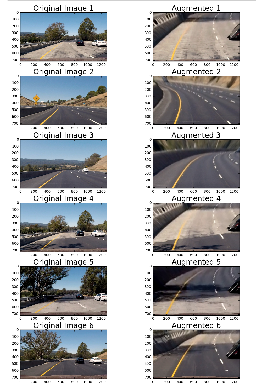
Now for this part I decided to transform before applying my thresholds on the image. (Contrary to how the helper functions are written). This was done with the getPerspectiveTransform and warpPerspective funtions.
Transform Points
| Source | Destination |
|---|---|
| 250, 700 | 250, 700 |
| 1200, 700 | 1200, 700 |
| 550, 450 | 300, 50 |
| 750, 450 | 1000, 50 |
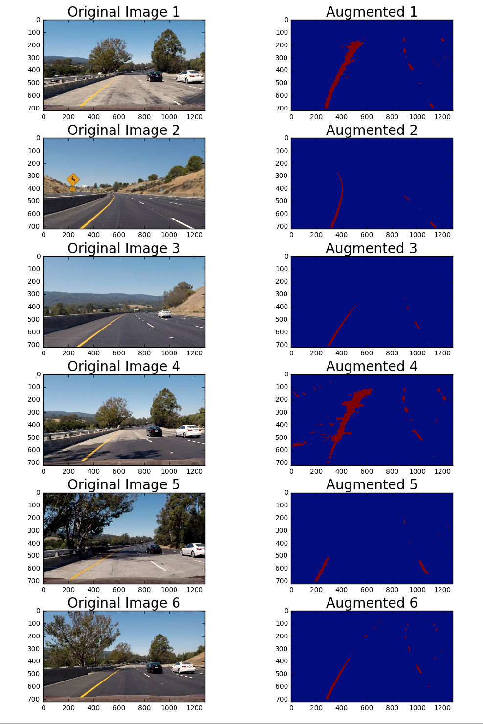
With the transform in place several pixel extractions were appliled and all combined into a final bitmask that is used in the next part. The labor for these functions is done with the respective color and gradient threshold funcitons. The layer and treshold type is provided in the table below.
Bit Extraction Table
| Color Layer Applied Too | Threshold Type |
|---|---|
| Red Layer (RGB) | Threshold |
| Value Layer (HSV) | Threshold |
| Yellow Extraction (HSV) | In Range |
| White Extraction (HSV) | In Range |
| White Extraction (HSL) | In Range |
| White Extraction (RGB) | In Range |
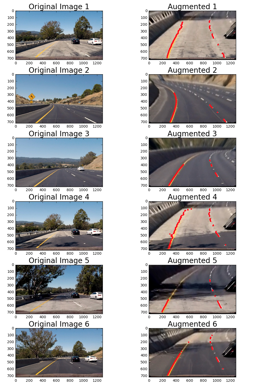
Lane lines were found by sliding a histogram window from the bottom of the bit mask to the upper 3/4 range. At each slice a point was indexed for were the highest density of pixels were found. See below for visualization.
Using the points gathered from the lane detction a 2nd order polynomial was fit to the data. With the new polynomial fit, new points were generated to simulate the entire lenth of the line. This can be seen below.
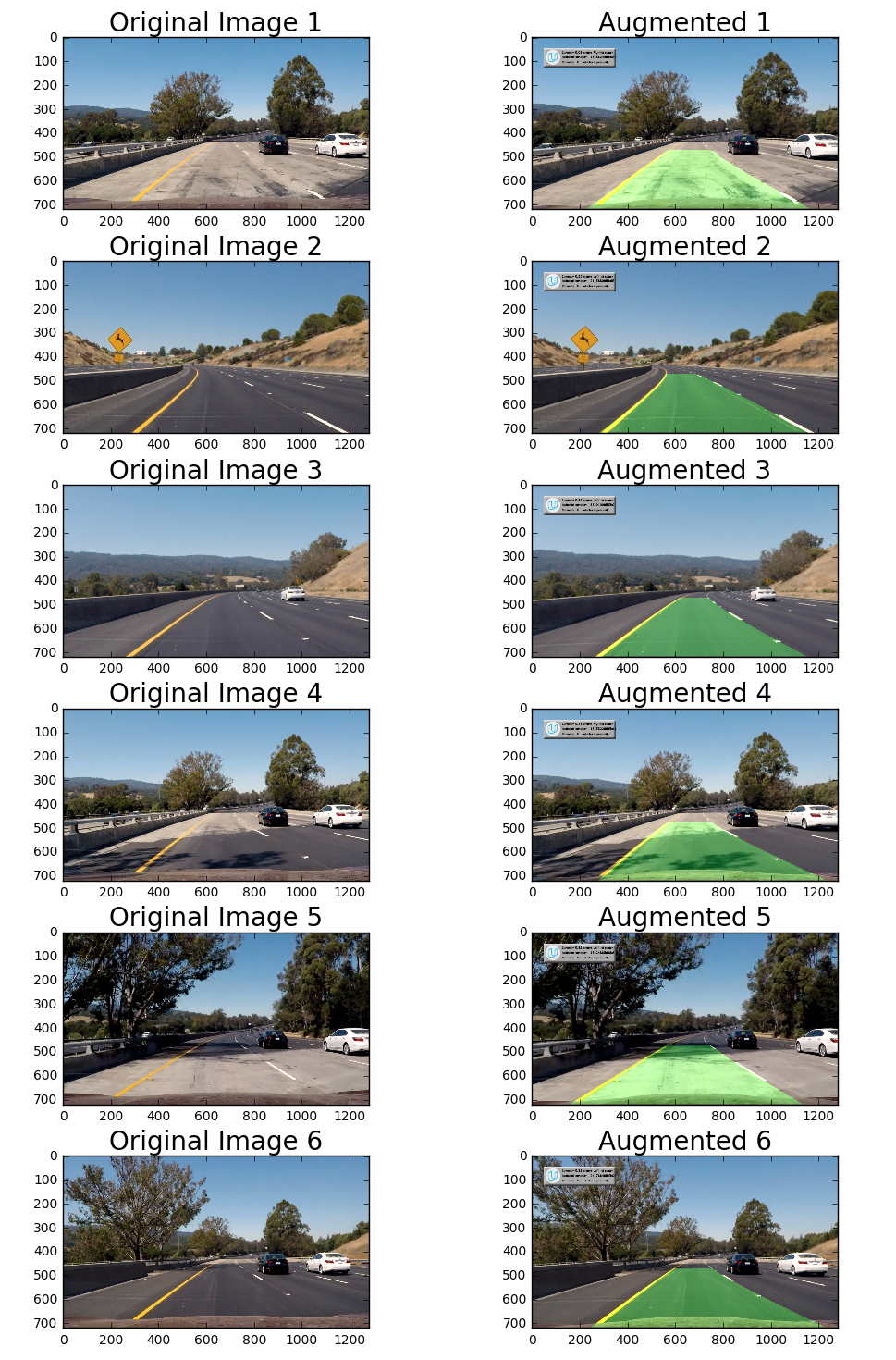
Lanes were imposed by taking the polynomial fit points and feeding them int opencv's poly fill to fill the polygon. From there the new polygon was then undistored, trucated, and imposed onto the rode as seen below.
8. Output Visual Display of Lane Boundaries and Numerical Estimation of Lane Curvature and Vehicle Position
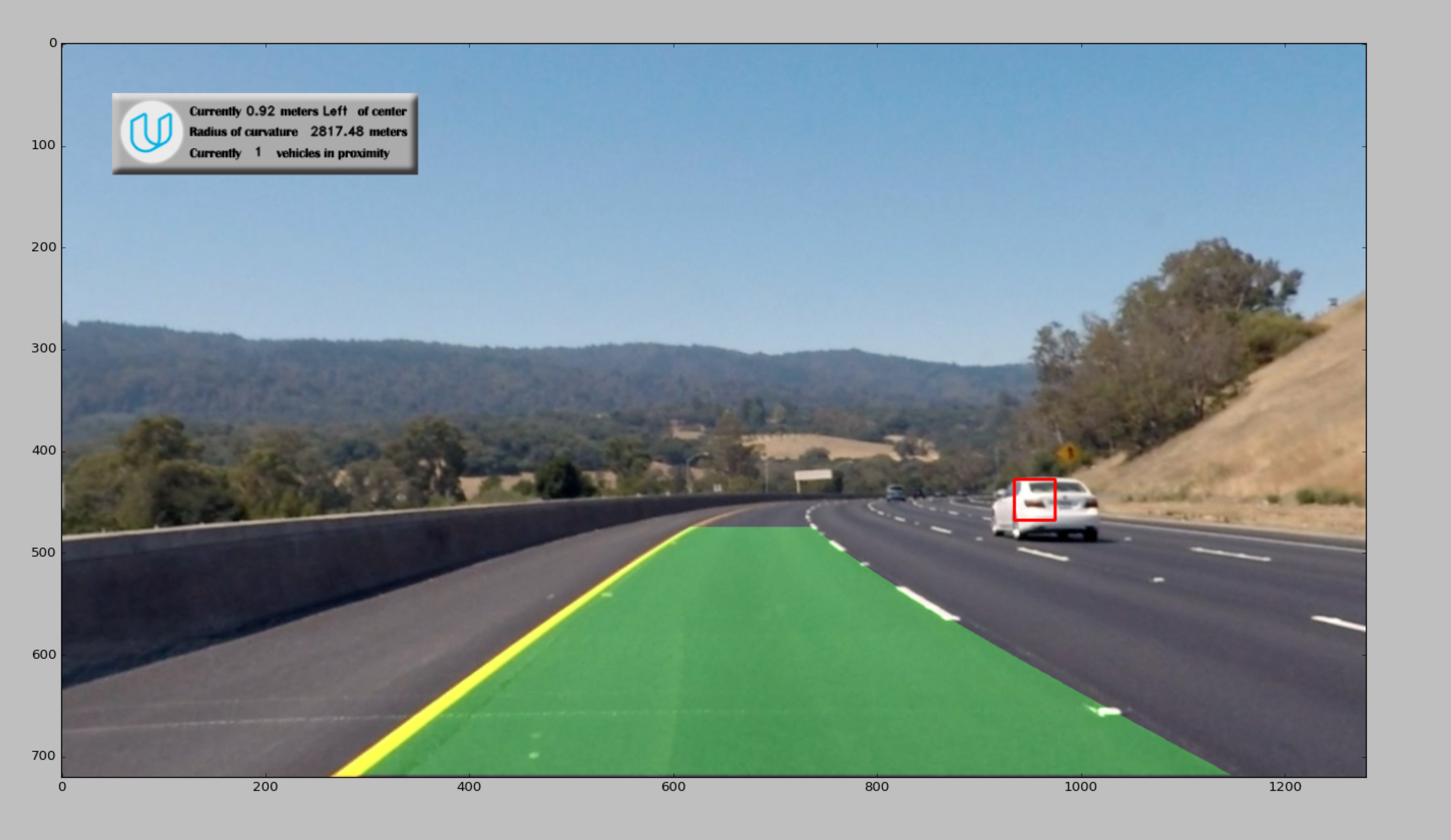
Lastly, distance from the center and the lane curvature were calculated from the bottom most pixels and updated every 10 frames and displayed in the dashboard.
A finalized frame is seen below:
This was an absoultly fantastic experience. At first the lanes were all over the place and very jittery. I applied techniques to help such as make sure that the polygon that comes after was of similar shape, I also ruled out polygons that failed to meet area requirements. When there errors arrose the last correct polygon was written instead.
Future improvents to avoid the algoritm from failing is a much cleaner bit mask extraction. When tested on the most difficult video the main problem was addtional noise creating points that ruined the polynomial fit. With more time a better bit mask extraction can be applied to enhace this algorithm.

