This library can be used to compute the magnetic field and the magnetic vector potential of filamentary current carriers in the form of a circular loop and straight segments. Arbitrary geometries of conductors can be approximated by a polygon along its contour and the connecting segments between the polygon vertices are modeled by straight segments. Finite-width conductors can be approximated by arranging multiple filaments throughout the cross section of the current carrier.

Please consider leaving a GitHub star if you like this software.

If you use this software for scientific work, we kindly ask you to cite the corresponding article:

@article{abscab_2023,
  title  = {{Biot-Savart routines with minimal floating point error}},
  author = {Jonathan Schilling and Jakob Svensson and Udo Höfel and Joachim Geiger and Henning Thomsen},
  journal = {Computer Physics Communications},
  pages = {108692},
  year = {2023},
  issn = {0010-4655},
  doi = {10.1016/j.cpc.2023.108692}
}

1. Implementations
2. API
   1. High-Level Methods
      1. Polygon Filament
      2. Circular Filament
   2. Low-Level Methods
      1. Straight Wire Segment
      2. Circular Wire Loop
3. Reference Outputs
4. Verification Procedure
   1. mpmath vs. Mathematica
   2. Test Points
   3. Reference Data

Various implementations are provided in this repository. Here is an overview:

Language	main abscab file	unit tests	demo code	parallel	CI
Java	ABSCAB.java	TestABSCAB.java	DemoABSCAB.java	✔️
C	abscab.h	test_abscab.c	demo_abscab.c	✔️
C++	abscab.cc	test_abscab.cc	demo_abscab.cc	✔️
Fortran	abscab.f08	test_abscab.f08	demo_abscab.f08	✔️
Python	abscab.py	test_abscab.py	demo_abscab.py	✖️

The Python implementation is deployed on PyPI: abscab-1.0.0

The Java implementation is available on Maven Central:

<dependency>
  <groupId>de.labathome</groupId>
  <artifactId>abscab</artifactId>
  <version>1.0.4</version>
</dependency>

The C++ implementation is available as an external package for use in Bazel:

# Accurate Biot-Savart routines with Correct Asymptotic Behaviour (C++)
# https://github.com/jonathanschilling/abscab
http_archive(
  name = "abscab_cpp",
  urls = [ "https://github.com/jonathanschilling/abscab-cpp/archive/refs/tags/v1.0.3.tar.gz" ],
  strip_prefix = "abscab-cpp-1.0.3",
)

The API consists of two levels. The high-level methods use the lower-level methods to evaluate the magnetic field and magnetic vector potential for a given current at given locations in global Cartesian coordinates. The lower level consists of methods for computing the normalized magnetic vector potential and magnetic field (i.e., only the geometric parts of the formulas) in normalized coordinates relative to the current carriers.

The high-level API constists of methods to compute the magnetic field and the magnetic vector potential of a polygon filament (current flows along straight wire segments from point to point along a polygon) and a circular filament.

SI Units are implied in the high-level interface. The geometric quantites are assumed to be specified in meters (m) and the current to be specified in Amperes (A). Then, the magnetic field is returned in Tesla (T) and the magnetic vector potential is returned in Tesla * meter (Tm).

The polygon describing the current carrier geometry is made up of the ordered list of points (vertices) along the polygon. A positive value of the current implies that the current flows along the polygon in the order of the points. The first and the last point of the polygon must coincide to model a closed loop. At least two points must be specified, which are then taken as start- and endpoint of a single straight wire segment.

The geometry of the polygon can be provided to the routines as an array.

• Java: double[][] vertices = new double[3][numVertices];
  The first dimension (3) is for the three components (x, y, z) of the Cartesian coordinates of the points.
  The second dimension (numVertices) is for the individual points along the polygon.
• C, C++: double vertices[3 * numVertices]; The geometry of the polygon is specified as a one-dimensional array.
  The order is (x_0, y_0, z_0, x_1, y_1, z_1, ..., x_n, y_n, z_n) where n = numVertices - 1.
• Fortran: real(wp), dimension(3, numVertices) :: vertices
  The first dimension (3) is for the three components (x, y, z) of the Cartesian coordinates of the points.
  The second dimension (numVertices) is for the individual points along the polygon.
• Python: arr(float) vertices: [numVertices][3: x, y, z]
  The first dimension (numVertices) is for the individual points along the polygon.
  The second dimension (3) is for the three components (x, y, z) of the Cartesian coordinates of the points.

The evaluation locations are provided to the routines as an array similarly shaped to the ones providing the polygon geometry (see above).

An optional parameter useCompensatedSummation (true by default) controls the use of Kahan-Babushka compensated summation when computing the superposition of the fields from the individual wire segments along the polygon. It can be set to false in order to use standard += summation into a single accumulation variable. This might be faster in some cases at the cost of giving up guaranteed accuracy.

The parallelized polygon routines allow to specify an optional parameter numProcessors specifying over how many threads the computation shall be parallelized. The parallelization is performed over either the number of source terms (number of wire segments along the polygon) or the number of evaluation locations, whichever is greater. This is done to ensure parallelization over as large chunks of computational work as possible for the most efficient use of available processors.

The magnetic vector potential of a polygon filament is computed using methods called vectorPotentialPolygonFilament.

The magnetic field of a polygon filament is computed using methods called magneticFieldPolygonFilament.

Furthermore, the geometry of the polygon can be provided via a callback function providing the coordinates of the i-th point along the polygon when being called with the point index i. This allows to compute the magnetic field and magnetic vector potential of polygon geometries that consist of so many points that holding them in memory simultaneously would not be possible. A suffix VertexSupplier is appended to these names (in C, Fortran and Python) to indicate the routines that accept a callback function for the polygon geometry.

The geometry of a current-carrying circular loop is described in terms of the origin of the loop, a normal vector and the radius of the loop.

The origin is a three-element vector which contains the Cartesian coordinates (x_0, y_0, z_0) of the center point of the loop in global coordinates.

The normal vector is a three-element vector which contains the Cartesian components (n_x, n_y, n_z) of a vector normal to the plane of the wire loop.

The radius of the loop completes the specification of the loop geometry.

A positive current implies that the current flows in clockwise direction along the wire loop when looking in positive direction along the normal vector. This is the usual direction of the tangential unit vector (e_phi) in a cylindrical coordinate system that has its z-axis aligned with the normal vector of the loop.

One call to the methods for the circular filament compute the magnetic field and magnetic vector potential at a number of evaluation locations due to the current in a single wire loop. Thus, for computing the magnetostatic quantities of a multi-winding coil, multiple calls (one for each winding of the coil) have to me made and the results need to be superposed to get the total fields of the coil.

The evaluation locations must be provided to the routines as an array.

• Java: double[][] evalPos = new double[3][numEvalPos];
  The first dimension (3) is for the three components (x, y, z) of the Cartesian coordinates of the locations.
  The second dimension (numEvalPos) is for the individual evaluation locations.
• C, C++: double evalPos[3 * numEvalPos]; The evaluation locations are specified as a one-dimensional array.
  The order is (x_0, y_0, z_0, x_1, y_1, z_1, ..., x_n, y_n, z_n) where n = numEvalPos - 1.
• Fortran: real(wp), dimension(3, numEvalPos) :: evalPos
  The first dimension (3) is for the three components (x, y, z) of the Cartesian coordinates of the locations.
  The second dimension (numEvalPos) is for the individual evaluation locations.
• Python: arr(float) evalPos: [numEvalPos][3: x, y, z]
  The first dimension (numEvalPos) is for the individual evaluation locations. The second dimension (3) is for the three components (x, y, z) of the Cartesian coordinates of the locations.

The magnetic vector potential of a circular filament is computed using methods called vectorPotentialCircularFilament.

The magnetic field of a circular filament is computed using methods called magneticFieldCircularFilament.

The low-level methods of this library are used to compute the geometric parts of the formulas for the magnetic vector potential and magnetic field of a straight wire segment and a circular wire loop. Normalized coordinates are used in a cylindrical coordinate system aligned with the axis of the wire segment in case of a straight wire segment and with the axis of the wire loop in the respective case of computing magnetostatic quantities for a circular wire loop.

Arguments to the routines listed below are rhoP and zP for the normalized radial and normalized vertical coordinates of the evaluation location, respectively.

Inside these routines, appropriate special-case formulations are used for given normalized coordinates of the evaluation location in order to maximize accuracy of the results.

The normalization factor used for the evaluation location in this case is the length L of wire segment.

The normalized magnetic vector potential of a straight wire segment only has a component A_z in the axial direction. This component is computed using routines named straightWireSegment_A_z(rhoP, zP). The return value of this method has to be multiplied by mu_0 * I / (2 * pi) to get the magnetic vector potential in units of Tm, where mu_0 is the vacuum magnetic permeability and I is the current along the wire segment.

The normalized magnetic field of a straight wire segment only has a component B_phi in the tangential/cylindrical direction around the wire segment. This component is computed using routines named straightWireSegment_B_phi(rhoP, zP). The return value of this methods has to multiplied by mu_0 * I / (4 * pi * L) to get the magnetic field in units of T, where mu_0 is the vacuum magnetic permeability, I is the current along the wire segment and L is the length of the wire segment.

The normalization factor used for the evaluation location in this case is the radius r of wire loop.

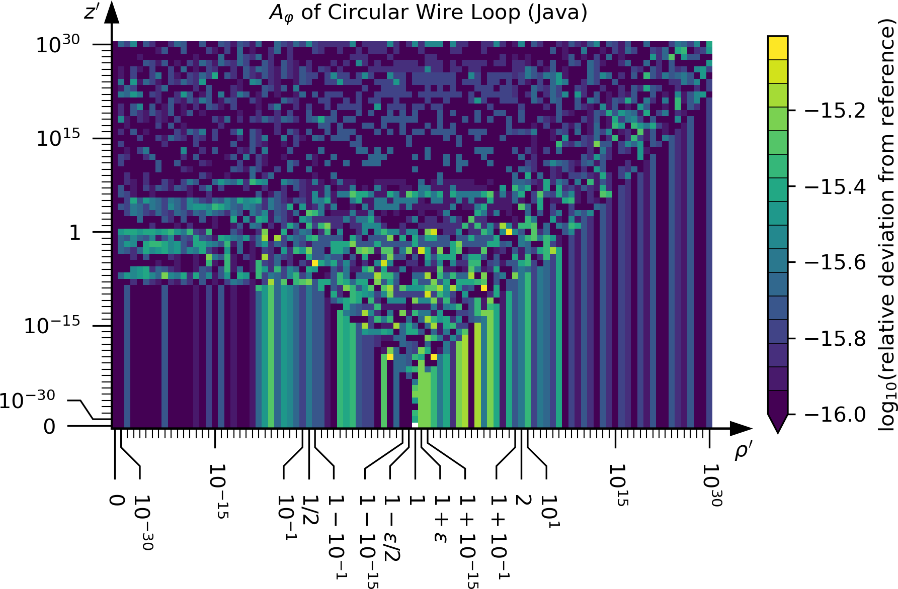
The normalized magnetic vector potential of a circular wire loop only has a component A_phi in the tangential/cylindrical direction of the wire loop. This component is computed using routines named circularWireLoop_A_phi(rhoP, zP). The return value of this methods has to multiplied by mu_0 * I / pi to get the magnetic vector potential in units of Tm, where mu_0 is the vacuum magnetic permeability and I is the current along the wire loop.

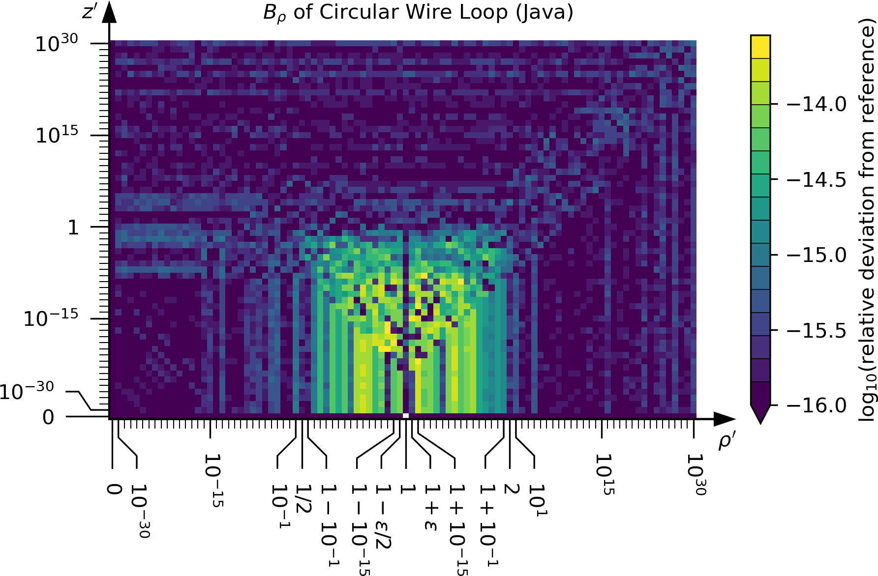
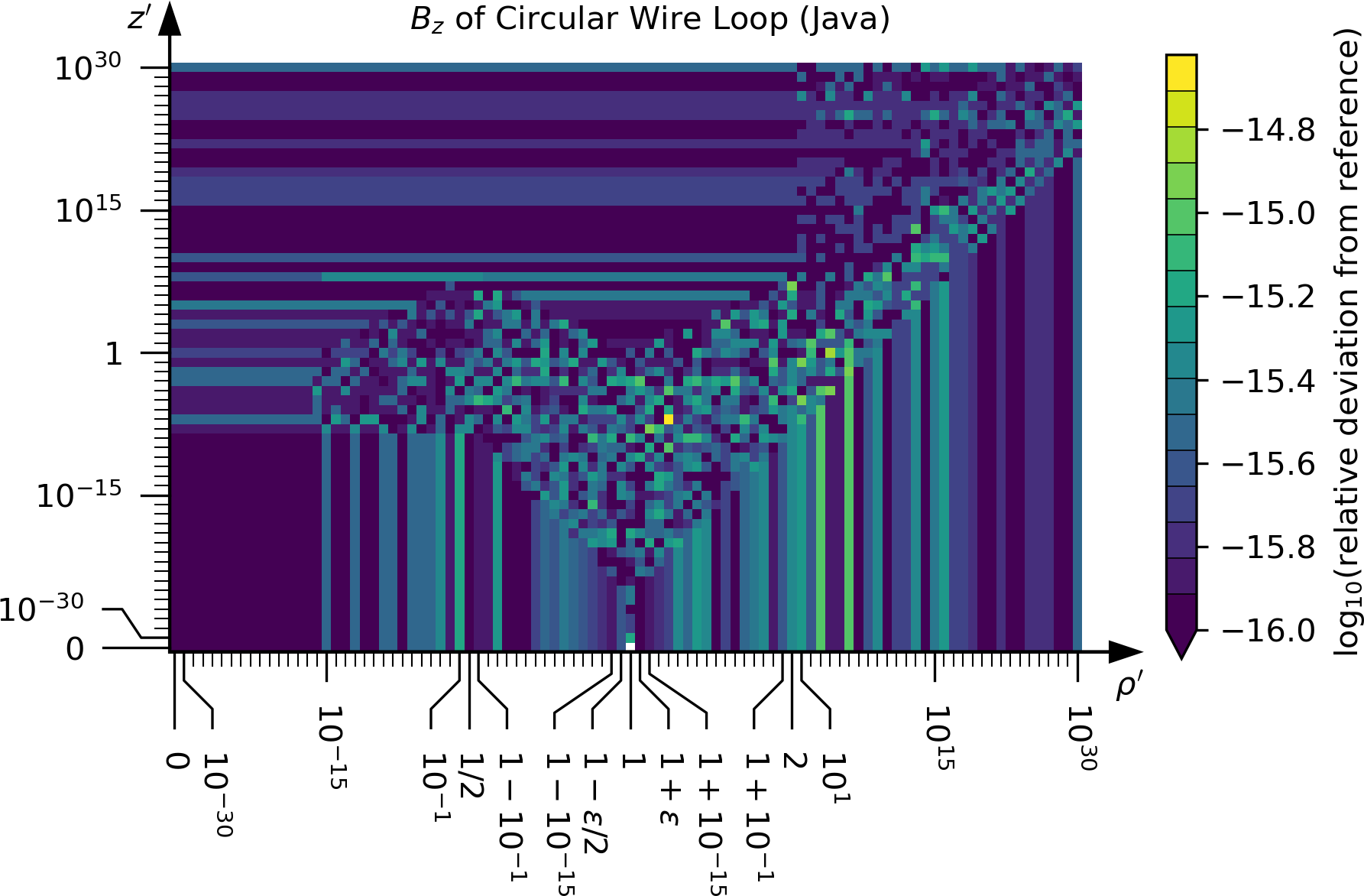
The normalized magnetic field of a circular wire loop has components B_rho and B_z in radial and vertical directions, respectively. The component B_rho is computed using routines named circularWireLoop_B_rho(rhoP, zP). The component B_z is computed using routines named circularWireLoop_B_z(rhoP, zP). The return values of these methods have to be multiplied by mu_0 * I / (pi * r) to get the magnetic field in units of T, where mu_0 is the vacuum magnetic permeability, I is the current along the wire loop and r is the radius of the wire loop.

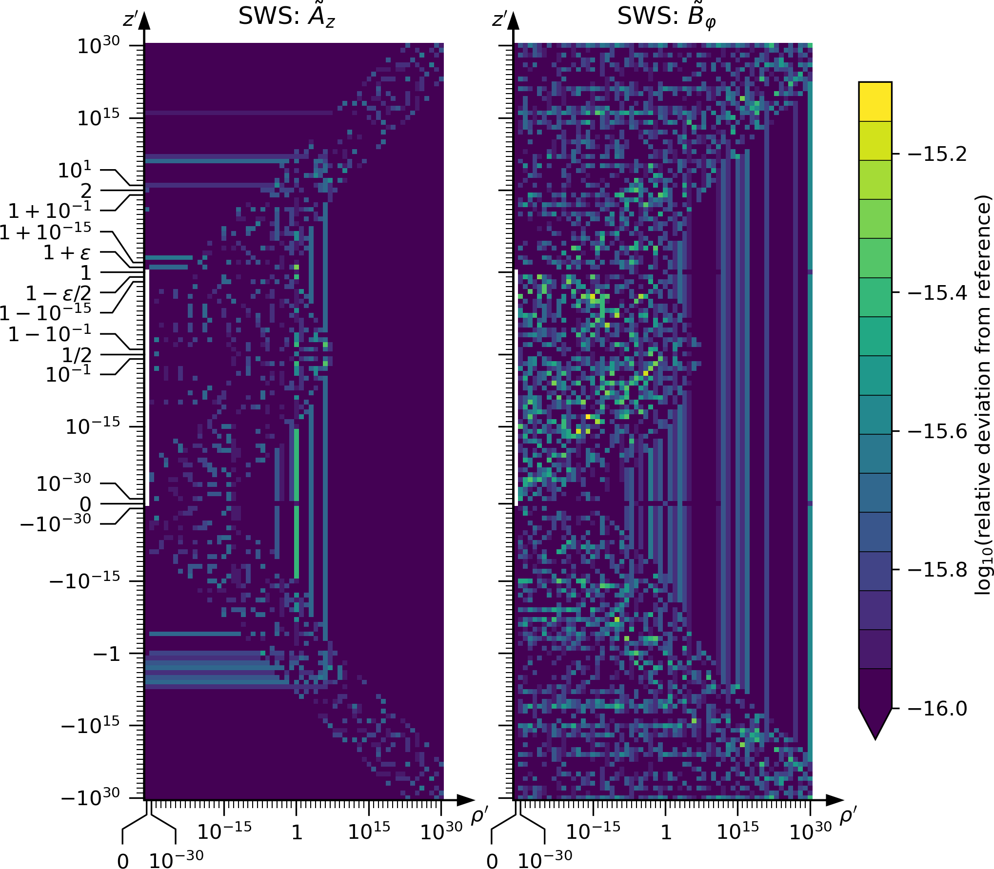
The following plots show the agreement between the Java implementation and the reference data computed using arbitrary-precision arithmetic.

First, the reference implementation using mpmath is verified against an implementation in Mathematica. For brevity, this is done on a reduced set of test points.

A set of test points is defined at which the implementations will be tested against the arbitrary-precision reference will be tested. These points are computed in Java, since it is a strictly-typed language and binaries are expected to produce platform-independent results. Nevertheless they are still of finite (64-bit) precision. The code to generate the test points is GenerateTestKnots.java.

The test points are saved into text files in src/test/resources:

• testPointsRpStraightWireSegment.dat contains the value of r' at which the straight wire segment methods are tested.
• testPointsZpStraightWireSegment.dat contains the value of z' at which the straight wire segment methods are tested.
• testPointsRpCircularWireLoop.dat contains the value of r' at which the circular wire loop methods are tested.
• testPointsZpCircularWireLoop.dat contains the value of z' at which the circular wire loop methods are tested.

Those above files are only provided to have a human-readable equivalent of the set of test points. The actual test point data read by the arbitrary-precision software is in testPointsStraightWireSegment.dat for the straight wire segment and in testPointsCircularWireLoop.dat for the circular wire loop.

The reference data (A_z and B_phi for a straight wire segment; A_phi, B_rho and B_z for a circular wire loop) is also available in the folder src/test/resources:

• refDataStraightWireSegment.dat was generated by computeReferenceStraightWireSegment.py and contains the quantities A_z and B_phi for a straight wire segment at all test points.
• refDataCircularWireLoop.dat was generated by computeReferenceCircularWireLoop.py and contains the quantities A_phi, B_rho and B_z for a circular wire loop at all test points.