- Motivation
- Dataset
- Yolo V1 Architecture
- Loss Function
- Evaluation Metrics
- Computational Resources
- How To Run
- Training Yolo V1
- Transfer Learning
- Models Comparision
- Validation With Our Own Images
- Conclusion And Future Work
- References
Problems and Challenges
The benefits of Autonomous vehicles
-
Greater road safety, reduce crash, and congestion,
-
Independence for people with disabilities (blind, old)
New potential risks.
-
Decision errors that may result in death and injury
-
Cybersecurity:
Critical Tasks to increase benefits and mitigate risks
- Object detection, drivable area segmentation, lane detection, deep detection, etc
Main Project Goal
-
Focus on traffic object detection (classification and localization)
-
Object detection is a crucial for object tracking, trajectory estimation, and collision avoidanc
Main Project Challenge
- Detect dynamic road elements (pedestrians, cyclist, vehicles) that are continuously changing location and behaviour under diverse lighting and background conditions
The Berkeley Deep Drive dataset contains a variety annotated images for 2D and 3D object detection, instance segmentation, lane markings, etc. For our project, we use the annotated images for 2D object detection. The dataset consists over 100.000 video clips of driving videos in different conditions. For 2D object detection, an extraction on 100.000 clips is done to obtain images and the annotations of the bounding boxes. The images are in RGB and have a size of 1280x720 pixels. The annotations are provided in a JSON file including:
- Bounding Boxes and the corresponding object class
- Weather
- Time of the day
- Scene The video clips from where the images are extracted are filmed in different parts of the USA.
 |
|---|
| Localization of Berkeley Deep Drive image recordings |
 |
 |
|---|---|
| Number of images in each category in validation data set | Number of images in each category in test data set |
 |
 |
|---|---|
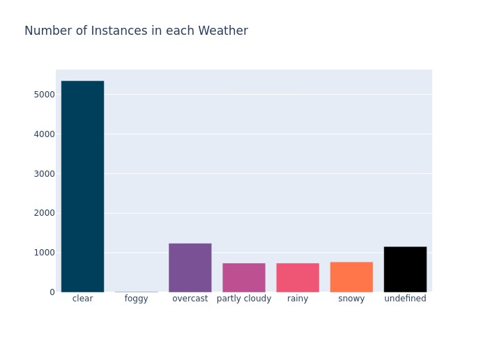
| Number of images in each weather condition in validation data set | Number of images in each weather condition in test data set |
 |
 |
|---|---|
| Number of images in each scene in validation data set | Number of images in each scene in test data set |
 |
 |
|---|---|
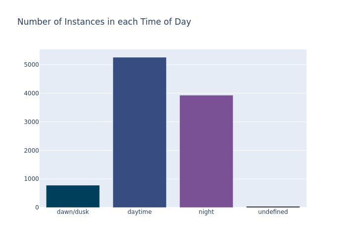
| Number of images in each time of the day in validation data set | Number of images in each time of the day in test data set |
We developed a python script to check wheter all the images in the diferent sets have an available annotation. Here is an example of the ouput when checking for the validation data:
Correct image-label mappings: 10000
Failed image-label mappings: 0
To run de script:
python data_mapping_analysis.py -j {JSON_PATH} -i {IMAGE_FOLDER_PATH}In addition, we provide a python script to analyse the distribution of annotation in the Berkeley Deep Drive dataset and generate the previous plots. To run it:
python db_analyse.py -j {JSON_PATH}You Only Look Once (YOLO) is an object detection model developed and published in 2015 by Redmon et al. The name is due to the fact that this algorithm is able to detect and recognize various objects in a picture only looking once at the input image, and requiring a single propagation pass through the network to obtain a prediction.
It is also important to mention that nowadays there exists a few improved versions of this model, but we have selected the YOLo v1 to reduce the complexity of the project and reduce the computational resources. YOLO uses an end-to-end convolutional neural network that takes as inputs RGB images of size 448x448. It outputs the corresponding bounding boxes and their class classification of all the detected objects in the input image.YOLO starts dividing the input image in a fixed number SxS grid:
After that, each of the SxS cells of the grid will be responsible to detect a maximum of 1 object of the image. It is important to know that we say that a cell is responsible for detecting an object if the center of the bounding box of this object is on the cell.
On the following example, the cell (4,3) would be the responsible for detecting the bike
In order to do this, YOLO v1 has an architecture consisting of 6 blocks combining convolutional layers with maxpooling layers and followed by 2 fully connected layers. Furthermore it applies the Leaky ReLu activation function after all layers except for the last one and uses dropout between the two fully connected layers in order to tackle overfitting.
The dimension of the last fully connected layer would be SxSx(B * 5 + C) where:
- S: Number of cells in which input image is divided
- B: Number of bounding boxes that will predict each cell (normally B=2, so each cell is responsible to detect 2 bounding boxes and then 1 is discarded)
- C: Number of classes of our dataset
So, for each cell of the image you have:
- 2 bounding boxes predicted: each bounding box has 4 numbers (center coordinates and width/height) and the number remaining is the probability of having an object inside this bounding box (P(Object)
- Class probabilities: For each of our dataset classes, we have the conditional probability (P(class 1 | Object)... P(class C | Object))
Number of parameters of our YOLO V1 model implemented from scratch:
================================================================
Total params: 85,630,247
Trainable params: 85,630,247
Non-trainable params: 0
----------------------------------------------------------------
Input size (MB): 2.30
Forward/backward pass size (MB): 316.92
Params size (MB): 326.65
Estimated Total Size (MB): 645.87
----------------------------------------------------------------The loss function in YOLO v1 is not one of the classic losses in neural networks. In this case, the loss is divided in different losses that we will see now: 1. Bounding box loss: This loss as the name suggests refers to the bounding box and it is divided into 2 different losses:
1.1. Bounding box centroid loss: This will be the distance of the center of the predicted bounding box and the ground truth bounding box but it is important to keep in mind that it is only computed when there actually exists an object on the studied cell. It is computed as follows:
1.2. Bounding box size loss: This one is computed as the distance of the width and height of the predicted bounding box and the ground truth bounding box but it is important to keep in mind that it is only computed when there actually exists an object on the studied cell. In this case we have to keep in mind also that it is computed the sqrt because otherwise larger bounding boxes would have more importance on this loss.
The formal formula is:
2. Object loss: This loss refers to the error that is done when assigning object probability and in the ground-truth there is an object. In other words, if there is an object on a particular cell, which is the difference between the P(Object) and 1? It is computed as follows:
3. No Object loss: This loss refers to the error that is done when assigning object probability and in the ground-truth there is not any object. In other words, if there is not any object on a particular cell, which is the difference between the P(Object) and 0? It is computed as follows:
4. Class loss: In this last loss, we are computing the error made when assigning a class to a detected object, so it is pretty similar as the previous loss but in this case, we are looking at the P(Class i | Object). The formula is:
So, finally, if we add all these losses, we will obtain the loss of YOLO v1:
We used several metrics to evaluate our object detection model.
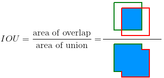
Intersection over Union is a metric used to measure the overlap between two vounding voxes. If the prediction is correct, the Iou is equal to 1. Therefore, the lower the IoU, the worse the prediction result.
In our project we used the IoU to classify the predictions as True Positives (TP), False Positives (FP) and False Negatives (FN):
- IoU >= 0.5: The prediction is classified as a True Positive (TP).
- IoU < 0.5: The prediction is classified as a False Positive (FP).
- When the model failed to detect and object in an image, the prediction is classified as a False Negative (FN)
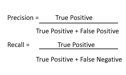
To evaluate the performance of the model, we used the previous tP, FP and FN classifications to compute the precision and recall of the model. On the one hande, the precision measures how accurate are our predictions, thus, the percentage of predictions that are correct. On the other hand, recall measures how good the model finds all the positives in a set of predictions.
Average precision computes the average precision values for recall value oer 0 to 1. To compute the Average Precision we find the area under the curve of the precision-recall curve.
The model was training using a GPU NVIDIA GeForce GTX 1080 Ti, with 10 GB of memory. Also, 2 CPUs were allocated and each CPU had 15 GB of memory.
 |
|---|
| GPU Information |
To run the training and evaluation of the model run, checking if we have an available GPU:
python -c 'import torch; print(torch.cuda.is_available())'
python main.py -i {PATH TO IMAGEçS -j {PATH_TO_LABELS}
The following optional arguments can be defined when running the code:
usage: main.py [-h] -j JSON_PATH -i IMGS [-b BATCH_SIZE] [-lr LEARNING_RATE] [-e EPOCHS]

Code to Train and Evaluate an 2D Object Detection Model (YOLO V1).

optional arguments:
  -h, --help            show this help message and exit
  -j JSON_PATH, --json_path JSON_PATH
                        Path to folder with JSON data.
  -i IMGS, --imgs IMGS  Path to foler with images. This path should contain 3 folder with val, train and test sets.
  -b BATCH_SIZE, --batch_size BATCH_SIZE
                        Batch Size. Default is 32.
  -lr LEARNING_RATE, --learning_rate LEARNING_RATE
                        Learning Rate. Default is 0.001
  -e EPOCHS, --epochs EPOCHS
                        number of epochs. Default is 100.
A slurm file example when executing in an HPC machine.
#!/bin/bash
#SBATCH --job-name yolov1
#SBATCH --cpus-per-task=2
#SBATCH --mem-per-cpu=15G
#SBATCH --gres=gpu:1

module purge
module load CUDA/11.1.1-GCC-8.3.0
export CUDA_VISIBLE_DEVICES=0

export LD_LIBRARY_PATH={PATH_TO_LD_LIBRARY_PATH}

source {PATH_TO_CONDA}/miniconda3/etc/profile.d/conda.sh
conda activate {PATH_TO_CONDA}/miniconda3/envs/AI

python -c 'import torch; print(torch.cuda.is_available())'
python main.py -i {PATH TO IMAGEçS -j {PATH_TO_LABELS}At first, we experienced exploiding gradients while training our network.
Exploding Gradients are a problem where large error gradients accumulate. This happened because our model was unstable and unacapable of learning from the training data.
 |
|---|
| Example plot of exploding gradients |
We observed this problem in it's extreme form, since the weight values resulted in NaN and can no longer be updated.
 |
|---|
| Example plot of exploding gradients until NaN values |
When training the network and finally solving the exploding gradients problem, the network simply would not converge on an acceptable solution. Despite the Loss values decreasing over the training stage, they were still too high, having values over 500.
 |
|---|
| Example plot of non-convergence of the loss |
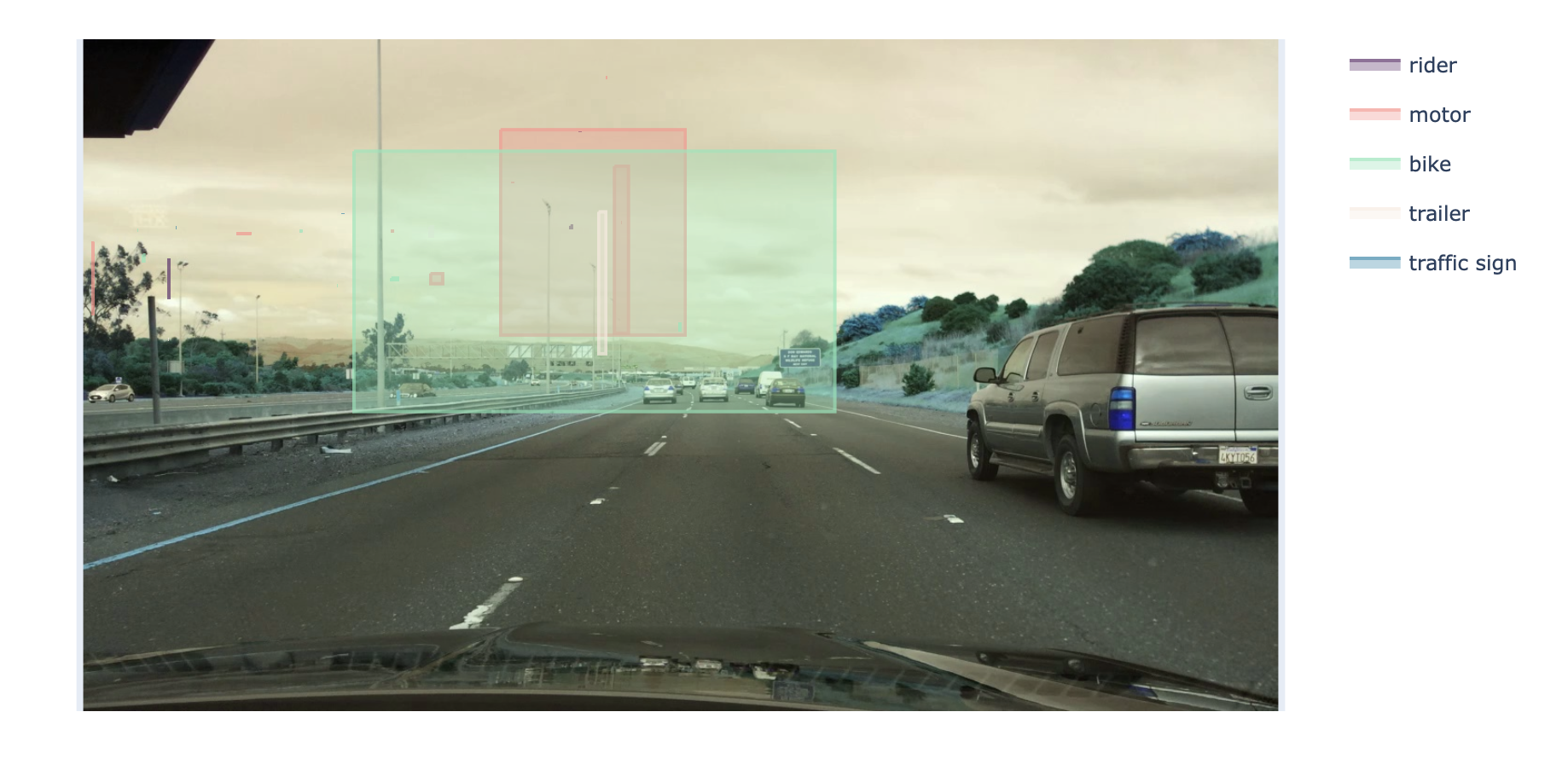
After training for a few epochs, we noticed that the predictions of the bounding boxes where only placed on the sides of the image, no predictions were made on the center of the image. This situation was repeated among all of the images that we checked the model with.
 |
|---|
| Example of image with bounding box predictions only on the sides. |
We suggested that the padding on the first convolutional layer of the model could be too big, and because of that the model was mainly focusing on the sides of the images. After changing the padding of the first layer, we observed that there were predictions also on the center of the images.
 |
|---|
| Example of image with bounding box predictions on the center. |
First of all, we will make a very quick introduction to Transfer Learning. The main idea of TL is using models already trained on our custom dataset. In order to do that, there are some steps that should be done:
- Select a model that performs the same (or a very similar) task as we want to do in order to take advantage of the features that the pretrained model already trained
- Select the backbone that we want for our model (it can be useful for faster predictions, for example)
- Load the parameters (weights and biases) from the pretrained model: In the case of pytorch, we have some models already pretrained for object detection (for instance Faster R-CNN and RetinaNet)
- Finetune the model to better adapt to our dataset: Finetuning the model means changing some parameters (or even some layers) so then we can train it again with our dataset. In our particular case, we needed to adapt the pretrained model to a different number of classes (as the models were previously pretrained with COCO (91 classes) and we have 13 classes)
- Train the model again for a few epochs: The idea is to train the model again but with our own data. Normally it is not needed to do it with the whole dataset but with a fewer subset (the main features are already learnt with the pretrained model and we only want to adapt it to our dataset)
- The "retrained" model will now do some better predictions on our dataset
The main advantages of doing transfer learning are the saving of computer and time resources but also the "no-need" to have huge datasets that normally are difficult/expensive to label.
As we have used the Pytorch environment on this project, we have taken advantage of some models already pretrained on pytorch and COCO dataset. So, we have selected 2 of the best performing models:
-
Faster R-CNN: This is the last algorithm of the trilogy (R-CNN, Fast R-CNN and Faster R-CNN) and the main idea is that there are 2 subnetworks (2-stage object detector):
-
Region Proposal Network: This network will be the responsible of purposing different regions in which may exist an object
-
Classifier: Here, the object classification will be done once the RPN has send to it some region proposals
-
- RetinaNet: This is a one-stage object detection model that utilizes a focal loss function to address class imbalance during training.
The Transfer Learning code is organized in this Google Colab in order to be more user-friendly. If we take a look at the colab, we will find it divided in 7 sections:
-
Prepare environment
In this first step, the idea was preparing the environment so that the code is perfectly executable. This means that this piece of code is responsible to download the needed data (images and annotations) but also installing all the needed packages to run each one of the cells in the notebook.
A small subset of the data has been prepared specifically for training and validating these models. It is important to note that the training dataset created for this purpose is a subset of the whole Deep Driving training dataset. Also, note that the training dataset is very small (120 images) because it is enough for understand perfectly how transfer learning works and for obtaining quite good results as we will see later.
-
Define DeepDriving Dataset Class
In order to pass the data through the data loader and the model, a new class is created where all the Dataset details are specified.
As always, this class has 2 main functions:
-
_init_ : Here, the images and json file are opened and saved as self objects
-
_getitem_: This is the most important part of the DeepDrivingDataset class, where the bounding boxes and labels are saved but also where the transformations are applied to the images. _getitem_ function will be the responsible to returning the images and targets.
In order to better understand the code, here we have an example of annotation:
 	{"name": "4c2cd55b-31488766.jpg",
 		"attributes": {
 			"weather": "clear",
 			"scene": "city street",
 			"timeofday": "daytime"
 			},
 		"timestamp": 10000,
 		"labels": [{
 			"category": "traffic light",
 			"attributes": {
 				"occluded": false,
 				"truncated": false,
 				"trafficLightColor": "green"
 				},
 			"manualShape": true,
 			"manualAttributes": true,
 			"box2d": {
 				"x1": 464.326734,
 				"y1": 243.551131,
 				"x2": 474.245106,
 				"y2": 270.00012
 				},
 			"id": 825728
 			}]
 		}
So, the annotations will be found on 'labels' section that's why we have the code
self.annotations.append(v["labels"])which creates a list with all the annotations found in an image ('v').
On the following piece of code, we can see how boxes and categories are saved (looking for them under the labels 'box2d' and 'category' respectively)
    for labels in self.annotations[idx]:
      if 'box2d' in labels:
        annotation = labels['box2d']
        lab = labels['category']
    	categories.append(self.label2idx[lab])
        #select the corners of the boxes for each axis. it should be a list with 4 values: 2 coordinates.
        boxes.append([annotation["x1"],annotation["y1"],annotation["x2"],annotation["y2"]])
Finally, a dictionary 'target' is created containing boxes and labels for the studied image and the image is converted to tensor (in order to apply the model directly to that).
-
-
Download the Pretrained model
We could say that this section is one of the most important parts of the code. Here, the idea is downloading pretrained models that are in PyTorch and adapt them to our dataset. In order to do that, we have chosen 2 models:
3.1. Faster-RCNN: As we have seen this model on the Postgraduate Lessons, we know that this model works pretty good and we had the advantage that it is already pretrained in PyTorch with different backbones. But before we continue, let's define better what is a backbone of the object detection model:
A backbone is a pre-trained model (it can be pre-trained on ImageNet, ResNet50, MobileNet...) that works as a feature extractor, which gives to the model a feature map representation of the input. So, once the model has the backbone defined, it has to perform the actual task which is object detection in our case. Summarizing, a backbone is very useful to make the network learn faster the object detection task.
3.2. RetinaNet: We also used this model but in this case we only have the pretrained model with ResNet50 backbone
It is important to note that in order to run this peace of code, 2 parameters need to be defined:
- backb: 1, 2 or 3 for "MobileNet v3", "ResNet 50" or "MobileNet v3-320" respectively
- pret_model: "FasterRCNN" or "RetinaNet" depending on the pretrained network for object detection that we want to use
-
Create the training function
The training function is surprisingly one of the simplest functions in this notebook. It is only needed to take into account that we have to perform the usual steps:
- Set optimizer gradients to zero before starting backbpropagtion
- Save loss from model in order to monitor the loss evolution
- Perform backpropagation to update the weights and biases
- Do an step of the optimizer so the optimizer iterates over all parameters
-
Create the evaluation function
The evaluation function is much more complicated than the training one because here we compute different metrics to obtain the Mean Average Precision (mAp) of each epoch. Step by step:
- Use the model to obtain the bounding boxes predicted
- Perform NonMaximumSupression (object detection technique that aims at selecting the best bounding box out of a set of overlapping boxes) on the Bounding Boxes predicted so we do not have a lot of overlaping bboxes. In order to do NmS, we use an IoU threshold of 0.2 but it can be changed.
- After that, we select boxes, scores and labels of the filtered bounding boxes and we start working only with this subset.
- Next, a loop is done over the 13 categories of our dataset. For each category, we see if there are Ground Truth Bounding Boxes and Predicted Bounding Boxes. If it is the case, we compute the IoU between all the GT boxes vs all the predicted ones and we keep the one with highest IoU.
- If the highest IoU is greater than the IoU threshold defined, we have a True Positive; otherwise, we will have a False Positive.
- We compute the total of TP and FP for each class and then the recall and precision.
- Then, we use the function
torch.trapzin order to compute the area under the curve of precision-recall. The average of all the areas (one for each category) is computed and showed as the Average Precision of the current image. - At the end of the epoch, the Mean of the Average Precision of all the images is computed and printed as mAP of the epoch.
-
Training Loop (with evaluation included)
Finally we have the training loop, where for each epoch it performs the training (setting the model to model.train() and using the
trainfunction explained on point 4 and the validation (setting the model to model.eval() and using theevaluatefunction explained on point 5.After each epoch, the model is saved on the folder 'models' and the predictions on a folder called predictions_epochx and the file names will specify which model has been used.
-
Performing only the evaluation (loading the models already pretrained with TL)
This section is almost the same as the previous one. The main difference is that here, the models are loaded already trained so you do not have to spend time training them. In order to download the models we had to upload them on our Google Cloud Storage in a specific public bucket created for this purpose.
-
Testing the models with slef-uploaded images
On this last section, the user can upload his/her own images from a local environment for testing the different models trained. In order to do that, first it is used the google.colab package and the
files.upload()function.Once the image is uploaded, it is passed through the model selected on the previous cells with the self-defined testing function. After executing the function we will obtain an image saved on 'predictions' folder with the bounding box predicted drawn on it.
In this section we will compare the different pretrained models used with transfer learning methods in order to see which ones have the best performance.
We will start with the training results. We have trained the 4 models/backbones with 120 images, 3 epochs and a batch size of 5. So, first we will compare the different backbones used for FasterRCNN because we have the same loss types here:
| Loss Type | Epoch | FRCNN-MNetV3 | FRCNN-ResNet50 | FRCNN-MNetV3-320 | RetinaNet-ResNet50 |
|---|---|---|---|---|---|
| Classifier Loss | Epoch 1 | 0.782 | 0.806 | 0.699 | 0.628 |
| Classifier Loss | Epoch 2 | 0.378 | 0.444 | 0.370 | 0.440 |
| Classifier Loss | Epoch 3 | 0.333 | 0.352 | 0.206 | 0.303 |
| Box Regression Loss | Epoch 1 | 0.544 | 0.611 | 0.298 | 0.388 |
| Box Regression Loss | Epoch 2 | 0.446 | 0.541 | 0.258 | 0.332 |
| Box Regression Loss | Epoch 3 | 0.420 | 0.524 | 0.158 | 0.305 |
| ObjectNess Loss | Epoch 1 | 0.130 | 0.226 | 0.105 | - |
| ObjectNess Loss | Epoch 2 | 0.071 | 0.088 | 0.092 | - |
| ObjectNess Loss | Epoch 3 | 0.055 | 0.058 | 0.102 | - |
| RPN Loss | Epoch 1 | 0.125 | 0.237 | 0.161 | - |
| RPN Loss | Epoch 2 | 0.112 | 0.183 | 0.145 | - |
| RPN Loss | Epoch 3 | 0.103 | 0.163 | 0.130 | - |
We can see that all the losses tend to decrease but we can highlight the classifier loss which normally tends to decrease around a 50% from the first epoch to the second one. Also, we should note that in general, all the losses are really small, this is due to the fact that these models are already trained so it is normal that we do not have very high losses. Another interesting thing to see is that the RPN and box regression losses are the ones that decrease more slowly, it can also be happening because the models already know to detect objects but they have to learn the exact classes which may be different from the ones used in the pretrained models.
Finally, if we take a look at the average loss per epoch (and also compared with RetinaNet average loss):
| Loss Type | Epoch | FRCNN - MobileNetV3 | FRCNN - ResNet50 | FRCNN - MobileNetV3-320 | RetinaNet-ResNet50 |
|---|---|---|---|---|---|
| Average Loss | Epoch 1 | 0.395 | 0.470 | 0.316 | 0.508 |
| Average Loss | Epoch 2 | 0.252 | 0.314 | 0.216 | 0.386 |
| Average Loss | Epoch 3 | 0.228 | 0.274 | 0.149 | 0.304 |
We can see that all the losses tend to decrease and it seems that FasterRCNN with MobileNetV3-320 as backbone offers the best results but let's see what happens on the evaluation of the model with validation images.
First of all we will take a look at the Mean Average Precision of the 3 validation epochs for each of the tested models:
| Epoch | FRCNN - MobileNetV3 | FRCNN - ResNet50 | FRCNN - MobileNetV3-320 | RetinaNet-ResNet50 |
|---|---|---|---|---|
| Epoch 1 | 0.430 | 0.517 | 0.301 | 0.498 |
| Epoch 2 | 0.476 | 0.457 | 0.219 | 0.377 |
| Epoch 3 | 0.358 | 0.457 | 0.223 | 0.461 |
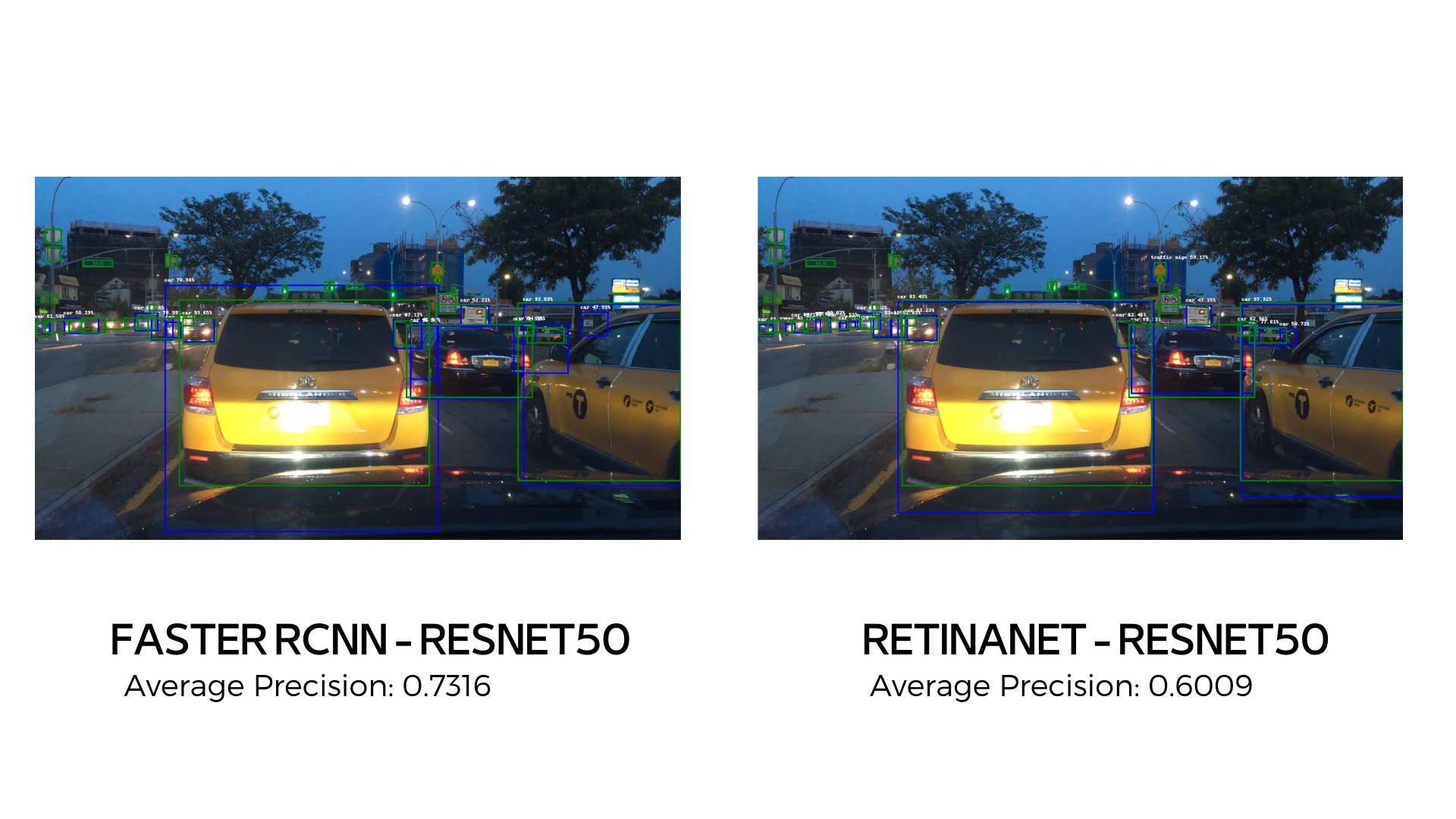
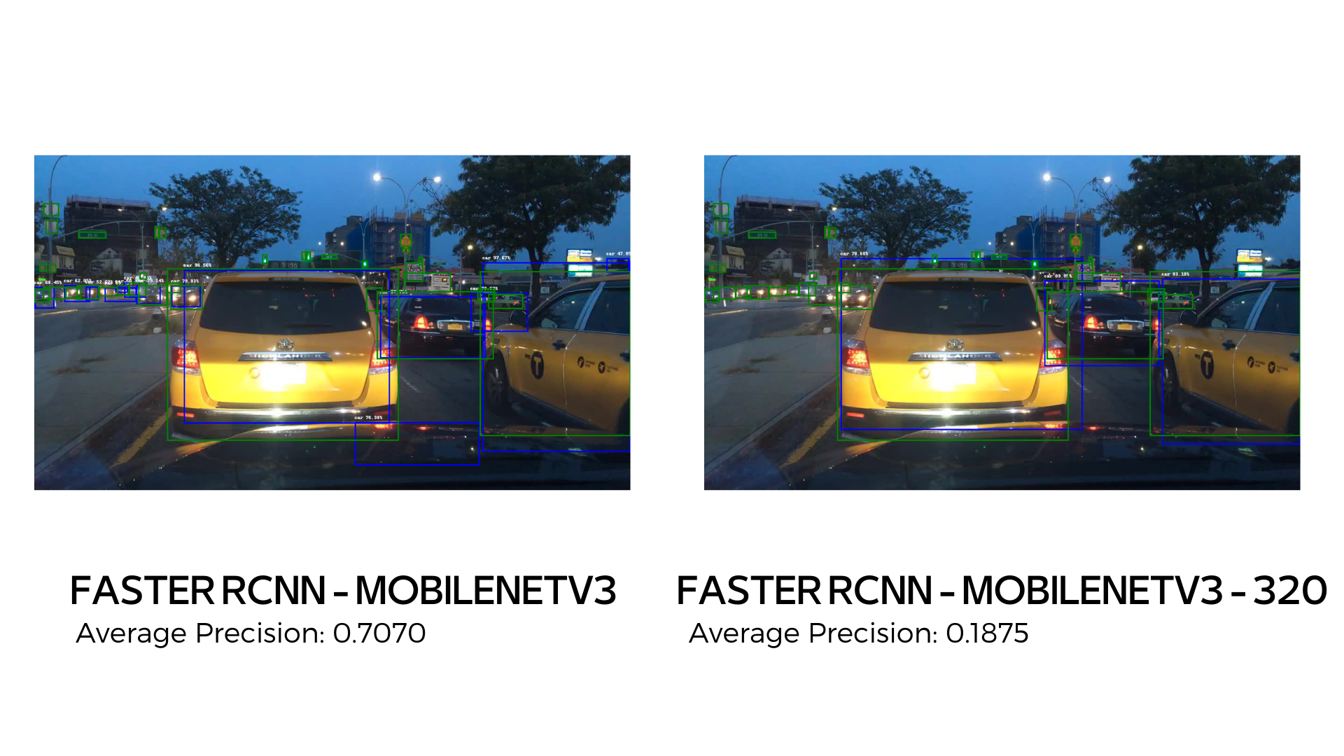
Here we can see that in most of the cases, the Mean Average Precision is better on the first epoch. However, it can be seen that the results are much better than the ones obtained in YOLO v1 from scratch. Furthermore, if we only look at these values, it may seem very small but let's see some images on the first epoch:
 |
|---|
| Comparison between ResNet backbone in FasterRCNN vs RetinaNet |
 |
|---|
| Comparison between FasterRCNN in MobileNetV3 vs MobileNetV3-320 |
On these first images, we can see that the models are detecting quite good the main elements of the image, but it can be seen that MobileNetV3-320 may have less precission and also less accuracy when detecting objects that are a more small (cars at the left). Also, any model is able to detect the traffic signs propery except for the RetinaNet which detects the traffic sign on the right. However it has a lower Average Precision than the Faster RCNN with ResNet50.
 |
|---|
| Comparison between ResNet backbone in FasterRCNN vs RetinaNet |
 |
|---|
| Comparison between FasterRCNN in MobileNetV3 vs MobileNetV3-320 |
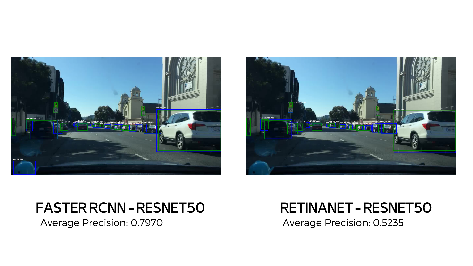
Now, again MobileNetV3-320 is the worst model detecting the objects of the image but at least it detects the bigger objects. On the other hand, RetinaNet with ResNet 50 is the only model capable to detect traffic signs on the left.
Now, let's see a very interesting example where we will compare the same image on the different validating epochs. As we have seen that the FasterRCNN model with MobileNetv3-320 backbone is not working well, we are not going to pay attention to this one but to the others.
 |
|---|
| Comparison between FasterRCNN in MobileNetV3 in the different epochs |
Here, it can be seen that there are not so much differences between the first and the second epoch. On the second epoch, as our threshold is 0.2, as there are less detections, the AP is better but in fact it does not mean that our model is performing better but we should need to adjust the IoU threshold. The main difference comes on the 3rd epoch where the model seems to have learnt more labels (person and traffic sign) and it starts detecting these objects. Again, the Average Precision is worse because there are much more positives (True or False) and it increases the probability of failing.
 |
|---|
| Comparison between FasterRCNN in ResNet50 in the different epochs |
On the case of FasterRCNN with ResNet50 backbone, we start looking differences at the 2nd epoch where it seems that the model has already learnt the traffic signs labels. In the 3rd epoch, it starts to understand what is a person and so, it does some detections of people. Also here, we can note that the average precision decreases as the model learns new labels.
 |
|---|
| Comparison between RetinaNet in ResNet50 in the different epochs |
Finally, we can see that RetinaNet with ResNet50 backbone starts to "learn" detecting people at the 2nd epoch and traffic signs at the 3rd epoch. Also it can be seen the problem of Average Precision due to the fact that it increases the number of available labels.
As said before, at the last section of the Google Colab, the user can upload an image and the selected model will predict the resulting bounding boxes and labels. Here, we can see an example of a photo took by ourselves and passed through the model:
 |
|---|
| Self-user image passed through FasterRCNN with ResNet 50 |
We can see that the model is working very well, detecting mainly the cars, traffic signs and traffic lights.
In our project we implemented and trained a one stage detector YOLO and two stage detector Faster R-CNN on the BDD 100K dataset in the context of of autonomous vehicles.
The main result: we just explore one of the main critical tasks, namely object detection.
Since we used the first version of YOLO in this project, in the future we must experiment with newer models, for instance the most recent versions of YOLO,
In the Future we will need to explore these three tasks simultaneously. We may add a four critical task: deep detection. This would allow us to reach performance with high accuracy and high FPS which are suitable for the goal of autonomous driving.
Since autonomous vehicles take decisions involving matters of life and death, we will have to find new ways to train the autonomous vehicle to make these complex decisions.
Generally we would need higher precision and real-time driving perception system that can assist the autonomous vehicle in making the reasonable decision while driving safely.
Gene Lewis. Object detection for autonomous vehicles, 2014.
Jason Brownlee. A gentle introduction to object recognition with deep learning. Machine Learning Mastery, 5, 2019.
S. Ren, K. He, R. Girshick, and J. Sun, “Faster r-cnn: Towards realtime object detection with region proposal networks,” arXiv preprint arXiv:1506.01497, 2015
A. Bochkovskiy, C.-Y. Wang, and H.-Y. M. Liao, “Yolov4: Optimal speed and accuracy of object detection,” arXiv preprint arXiv:2004.10934, 2020
A. Paszke, A. Chaurasia, S. Kim, and E. Culurciello, “Enet: A deep neural network architecture for real-time semantic segmentation,” arXiv preprint arXiv:1606.02147, 2016
H. Zhao, J. Shi, X. Qi, X. Wang, and J. Jia, “Pyramid scene parsing network,” in Proceedings of the IEEE Conference on Computer Vision and Pattern Recognition (CVPR), July 2017
X. Pan, J. Shi, P. Luo, X. Wang, and X. Tang, “Spatial as deep: Spatial cnn for traffic scene understanding,” in Proceedings of the AAAI Conference on Artificial Intelligence, vol. 32, no. 1, 2018
Y. Hou, Z. Ma, C. Liu, and C. C. Loy, “Learning lightweight lane detection cnns by self-attention distillation,” in Proceedings of the IEEE/CVF International Conference on Computer Vision, 2019, pp. 1013–1021
C.-Y. Wang, A. Bochkovskiy, and H.-Y. M. Liao, “Scaled-yolov4: Scaling cross stage partial network,” arXiv preprint arXiv:2011.08036, 2020.
Joseph Redmon, Santosh Divvala, Ross Girshick, and Ali Farhadi. You only look once: Unified, real-time object detection. In Proceedings of the IEEE conference on computer vision and pattern recognition, pages 779-788, 2016.


