Askham et al. introduced the variable projection for the Dynamic Mode Decomposition (DMD).
This repository compares two implementations of the variable projection method for DMD (BOPDMD originally introduced by Sashidar and Kutz, VarProDMD) w.r.t. overall optimization runtime and signal reconstruction capabilities. BOPDMD reduces to the classic variable projection
if only one model is considered. The preselection $\widetilde{\boldsymbol{X}} \in \mathbb{C}^{n \times k}$ of original measurements $\boldsymbol{X} \in \mathbb{C}^{n \times m}, k < m$ can in some cases accelerate the optimization. The preselection is achieved by QR-Decomposition with Column Pivoting. This project mainly focuses on the python implementations.
Note that in Python the execution times vary, due to system calls or waiting for resources.

The easiest way to run the scripts is to use VSCode's devcontainer capability. The project was tested on Ubuntu 22.04 (which also served as a host system for the devcontainers) with the Python3.11 interpreter.

To visualize the results some prerequisites are necessary.
First, download this repository and execute the following commands

cd /path/to/repository
python3.11 -m pip --user install -e .

For proper visualization of the results make sure LaTex is installed.
For a minimal installation open another command line window and execute

sudo apt update
sudo apt upgrade -y
sudo apt install texlive-xetex cm-super dvipng -y

Open the repository, press CTRL + SHIFT + P, and type Devcontainers: Rebuild and Reopen in Container.
After everything is ready to run.

After the setup phase execute

run_mrse -o /path/to/output/

for running the spatiotemporal signal experiment. For further information, please type

run_mrse -h

For the more complex experiments e.g. type

run_ssim -f moving_points -o /path/to/output

For detailed information type

run_ssim -h

You may also modify the optimizer within the experiments. Within your specified path a subfolder with the name of the optimizer used for the experiment is created. Note that some of the experiments require a lot of time.
The experiments also artificially corrupt the original signal with noise. Further, different compression rates (library selection) are considered. The results are stored in a .pkl file.

After the experiments were run you can easily visualize the runtime statistics.
Here is an example of how to visualize the sea surface temperature experiment

visualize_stats -p output/lm/MRSE_highdim_100_linear.pkl

Here is a visualization of how the QR decomposition with Column Pivoting (greedily) selects samples of a spatiotemporal signal
in the original (highdimensional) space. The spatiotemporal signal is also utilized in the experiments (cf. section Spatiotemporal Dyamics).

Within the experiments, the library selection in general is performed in the projected
low dimensional space:

The formula on how to generate the spatiotemporal dynamics is described in section Spatiotemporal Dynamics.
The signal consists of $100$ measurements with $1024$ entries $\left(\boldsymbol{X} \in \mathbb{C}^{1024 \times 100}\right)$.
The compression is set to $c = 0.8$, hence $20$ samples are utilized for the optimization.

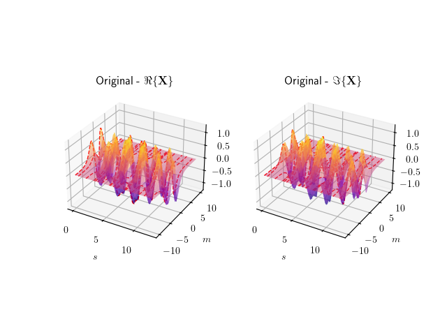Spatiotemporal signal: Real- and imaginary part of the signal. Dashed lines indicate library selection in high dimensional space.

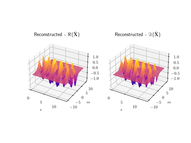Spatiotemporal signal: Reconstructed real- and imaginary parts of the signal. The reconstruction is performed with VarProDMD

All experiments consider different compressions and varying (zero-mean Gaussian) noise corruption with standard deviation $\sigma_{std} \in {0.0001, 0.001, 0.01}$.
Each experiment is executed 100 times. The optimization is performed in the projected (low-dimensional) space. The parameters used for the experiments are the default values of the different scripts (run_mrse, run_ssim).
Depending on the experiment either the mean/expected mean root squared error ($E\left[d\right]$) or the mean/expected Structural Similarity Index ($E\left[SSIM\right]$) is computed.
For $E\left[d\right]$ a low runtimes and a low error is desired. For $E\left[SSIM\right]$ a value close to 1 is desired, while also having a low expected runtime.

The formula for generating the spatiotemporal dynamics (taken from here):

Spatiotemporal Signal experiment: Expected runtime for BOPDMD and VarProDMD. Dashed ellipse indicate error- and time covariance. A dashed line is a collapsed ellipse. In this case only the execution times vary. VarProDMD uses Trust Region Optimization (TRF) during the experiment.

The oscillation experiment (taken from here) consists of $64$ complex $128 \times 128 px$ images.
Formula for generating the time dependend complex images:

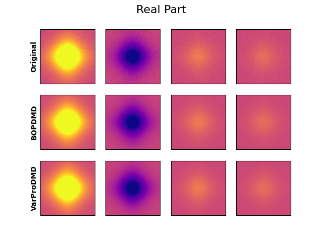Oscillations: The top row denotes the original real (noisy) signal. The bottom rows are the reconstructions of the different approaches.

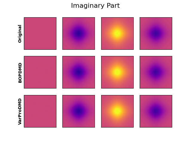Oscillations: The top row denotes the original imaginary signal. The bottom rows are the reconstructions of the different approaches.

Oscillations experiment: Expected runtime for BOPDMD and VarProDMD. VarProDMD uses Levenberg-Marquardt (LM) optimization within the experiment. The noise mainly influences the runtime (indicated by the dashed lines).

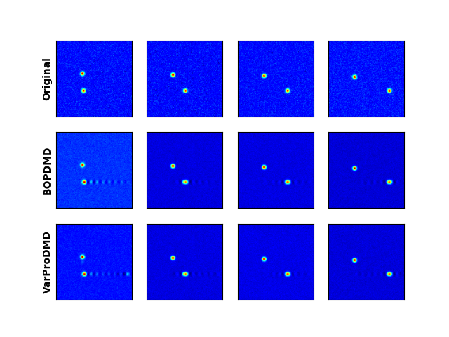
The moving point experiments consider $128$ samples and consist of $128 \times 128 px$ images.
The formula for generating the images was taken from here:

Moving Points experiment: The top row denotes the original (noisy) signal. The bottom rows are the reconstructions of the different approaches.

Moving Points: Expected runtime for BOPDMD and VarProDMD. Compression accelerates the optimization. BOPDMD however yields superior performance. VarProDMD uses LM optimization with Jacobian scaling during the experiment.