Travelling Salesman Problem in C language using Simulated Annealing.

Project created for Metaheuristic Algorithms course.

Computer Science, WPPT, Politechnika Wrocławska.

Output differs from optimum for about

• 1% for data size equals about 100 cities
• 6% for data size equals about 1000 cities
• 12% for data size equals about 10000 cities.

Times for appropriate tests are widely dispersed

• 1500 - 5000 ms for data size equals about 100 cities
• 4500 - 53000 ms for data size equals about 1000 cities
• 125000 - 235000 ms for data size equals about 10000 cities

Temperatures were chosen empirically by reading appropriate values from plots shown below. The point was to limit iterations of algorithm to only these values which have real impact for finding the best solution at the best time. Iterating at random solutions when temperature is too high is as unnecessary as computationally expensive searching for next better solution when temperature is enough low to make this searching unprofitable.

The first line contains an integer denoting n (number of cities). Each of the next n subsequent lines contains 3 integers i x y where i is city number and it is distinct integer of range 1...n, x and y are 2D euclidean coordinates of the city. And the last n+2 line contains an integer t describing maximal execution time.

Probability with which we accept worse solution than we got is calculated using this equation:

diff = newCycleLength - currentCycleLength

probability = exp(- diff / temperature)

It means that for listed differences, corresponding probabilities will be:

• diff = 0.01 * temperature, probability ~ 99%
• diff = 0.05 * temperature, probability ~ 95%
• diff = 0.1 * temperature, probability ~ 90%
• diff = 0.3 * temperature, probability ~ 74%
• diff = 0.5 * temperature, probability ~ 61%
• diff = 0.7 * temperature, probability ~ 50%
• diff = 1.0 * temperature, probability ~ 37%
• diff = 1.5 * temperature, probability ~ 22%
• diff = 2.0 * temperature, probability ~ 14%
• diff = 4.0 * temperature, probability ~ 2%

Starting solution is chosen randomly. The most probably solution will be called "average cycle" with length calculated using equation listed below. I noticed that high temperature leads cycle to hesitate around average cycle, so greedy algorithm for starting cycle is unnecessary. Starting temperature equals length of average cycle, it means

Tstart = averageCycleLength = numberOfCities * (sumOfAllEdgesLengths / numberOfEdges)

And with this temperature acceptance probability for 2 times worse solution will be 36%.

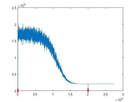
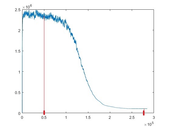
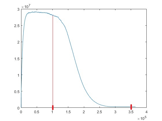
At the beginning lets analyze some plots and determine where it will be the best point to start, and to end to not waste time.

Cooling rate = 0.99995
X axis - number of iterations
Y axis - cycle length

As we can see here the best values are:

starting iteration = 0       (temperature = Tstart * 1 (coolingRate ^ 0))
ending iteration   = 200000  (temperature = Tstart * 0.000045389 (coolingRate ^ 200000))

The best values are:

starting iteration = 50000   (temperature = Tstart * 0.0821 (coolingRate ^ 50000))
ending iteration   = 275000  (temperature = Tstart * 0.000001067 (coolingRate ^ 275000))

And finally the best values here are:

starting iteration = 100000   (temperature = Tstart * 0.006737 (coolingRate ^ 100000))
ending iteration   = 350000  (temperature = Tstart * 0.0000000251 (coolingRate ^ 350000))

As we can see, the starting temperature are increasing by a constant factor whenever number of cities increase 10 times. We can define this by simple equation and precalculated value

factor = 0.0821
T = Tstart * pow(factor, log10(n) - 2.0)

The same way we can precalculate values to calculate ending temperature pretty fast

firstFactor = 0.000045389
factor = 0.0235
Tmin = Tstart * firstFactor * pow(factor, log10(n) - 2.0)

After modifications to iterations fit to appropriate start and end values, and draw values only between minimum and maximum of calculated cycle length we've got expected results

Above plots were depiciting 0.99995 cooling rate. What about the others? Interestingly, cycle length behaves same way at cooling rate 0.99999, and plots are the same for the same factors for starting and ending temperatures. It means that cooling rate which is 5th root of 0.99995 makes the same job but 5 iterations in place of single iteration of previous cooling rate which can give more precise solutions.

But the time the program runs is 5 times longer, with solution improvement for only about 30%. Of course cooling rate can be changed to calculate more accurate solutions, but for college use was limited to 0.99995.

I think I made pretty good analysis of simulated annealing metaheuristic. Everything consists of my own research on this subject. In my opinion these plots and their interpretation are enough to construct an efficient program.