1. Introduction
2. Applications
3. Prerequisites
4. Data collection
5. Understanding the data
6. Text Cleaning
7. Preparing the training and test set
8. Image Preprocessing - Image Features Extraction using Transfer Learning (ResNet-50 Model)
9. Preprocessing Captions
10. Image Captioning as Supervised learning problem and data preparation using Generator Function
11. Word Embeddings - Transfer Learning
12. Model Architecture
13. Model Training
14. Making Predictions
15. Conclusion

Caption generation is a challenging artificial intelligence problem where a textual description must be generated for a given photograph. Image captioning, i.e., describing the content observed in an image, has received a significant amount of attention in recent years. It requires both the methods - from computer vision to understand the content of the image and a language model from the field of natural language processing to turn the understanding of the image into words in the right order. Figure shown below can be used to understand the task of Image Captioning in a detailed manner.

The main challenge of this task is to capture how objects relate to each other in the image and to express them in a natural language (like English). Some real world scenarios where Image Captioning plays a vital role are as follows :

• Self driving cars — Automatic driving is one of the biggest challenges and if we can properly caption the scene around the car, it can give a boost to the self driving system.
• Aid to the blind — We can create a product for the blind which will guide them travelling on the roads without the support of anyone else. We can do this by first converting the scene into text and then the text to voice. Both are now famous applications of Deep Learning.
• CCTV cameras are everywhere today, but along with viewing the world, if we can also generate relevant captions, then we can raise alarms as soon as there is some malicious activity going on somewhere. This could probably help reduce some crime and/or accidents.
• Automatic Captioning can help, make Google Image Search as good as Google Search, as then every image could be first converted into a caption and then search can be performed based on the caption.

Image captioning is an application of one to many type of RNNs. For a given input image model predicts the caption based on the vocabulary of train data using basic Deep Learning techniques. So familarity with concepts like Multi-layered Perceptrons, Convolution Neural Networks, Recurrent Neural Networks, Transfer Learning, Gradient Descent, Backpropagation, Overfitting, Probability, Text Processing, Python syntax and data structures, Keras library etc is necessary. Furthermore, libraries such as cv2, Numpy , keras with Tensorflow backend must be installed. I have considered the Flickr8k dataset - Kaggle Flickr8k Dataset for this project.

There are many open source datasets available for this problem, like Flickr 8k (It is a collection of 8 thousand described images taken from flickr.com), Flickr 30k (containing 30k images), MS COCO (containing 180k images), etc. But a good dataset to use when getting started with image captioning is the Flickr8K dataset. The reason is because it is realistic and relatively small so that we can download it and build models on our workstation using a CPU(preferably GPU). Flickr8k is a labeled dataset consisting of 8000 photos with 5 captions for each photos. It includes images obtained from the Flickr website. The images in this dataset are bifurcated as follows:

• Training Set — 6000 images
• Validation Set — 1000 images
• Test Set — 1000 images

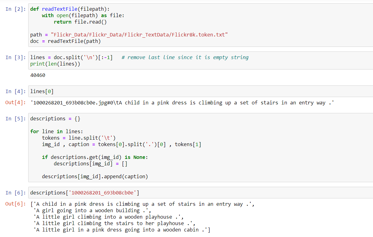
In the downloaded Flickr8k dataset, along with Images folder there would be a folder named 'Flickr_TextData' which contains some text files related to the images. One of the files in that folder is “Flickr8k.token.txt” which contains the name of each image along with its 5 captions.

Thus every line contains the #i , where 0≤i≤4 , i.e. the name of the image, caption number (0 to 4) and the actual caption.

Firstly, we will create a dictionary named “descriptions” which contains the name of the image (without the .jpg extension) as keys and a list of the 5 captions for the corresponding image as values.

Before we proceed with text cleaning, lets visualize an image using Matplotlib library.

When we deal with text, we generally perform some basic cleaning like lower-casing all the words (otherwise “hello” and “Hello” will be regarded as two separate words), remove special tokens or punctuation-marks (like ‘%’, ‘$’, ‘!’, etc.), eliminate words containing numbers (like ‘hey199’, etc.) and in some NLP tasks, we remove stopwords and perform stemming or lemmatization to get root form of the word before finally feeding our textual data to the model. In this project, while text cleaning :

• Stop words have not been removed because if we don’t teach our model how to insert stop words like was, an, the, had , it would not generate correct english.
• Stemming has not been performed because if we feed in stemmed words, the model is also going to learn those stemmed words . So for example, if the word is ‘running’ and we stem it and make it ‘run’ , the model will predict sentences like “Dog is run” instead of “Dog is running”.
• All the text has been converted to lower case so that ‘the’ and ‘The’ are treated as the same words.
• Numbers, Punctuations and special symbols like ‘@‘, ‘#’ and so on have been removed, so that we generate sentences without any punctuation or symbols. This is beneficial as it helps to reduce the vocabulary size. Small vocabulary size means less number of neurons and hence less parameters to be computed and hence less overfitting.

After text cleaning, write all these captions along with their image names in a new file namely, “descriptions.txt” and save it on the disk.

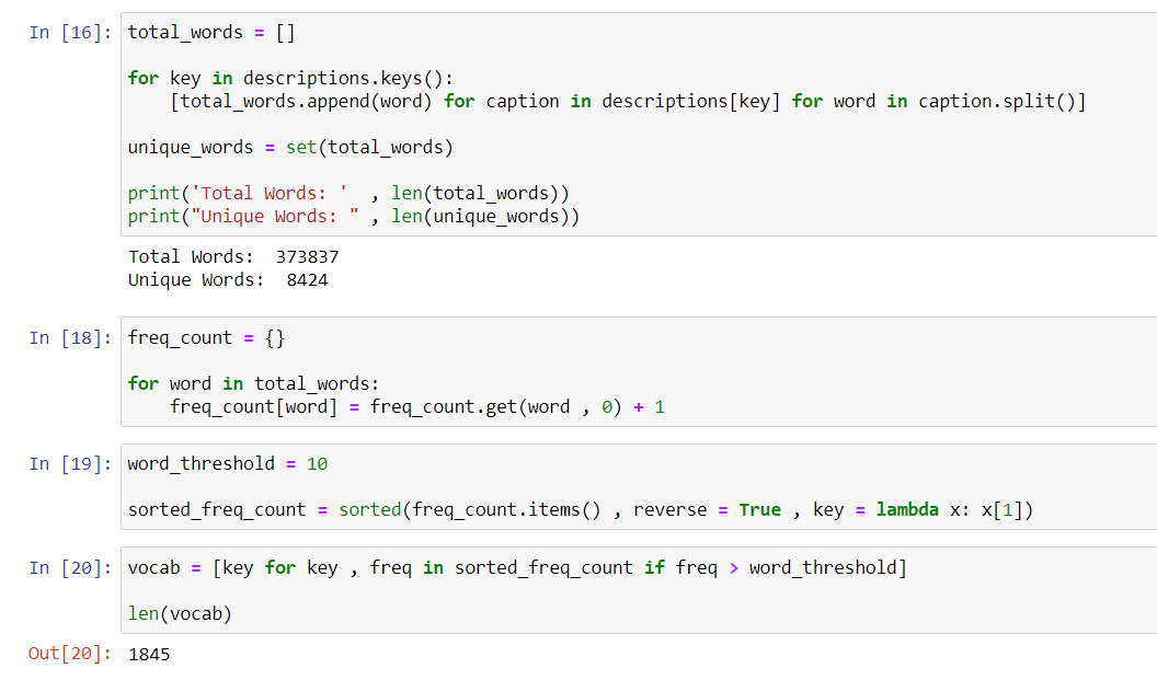
Next we will create a vocabulary of all the unique words present across all the 8000*5 (i.e. 40000) image captions in the dataset. Total unique words that are there in the dataset are 8424. However, many of these words will occur very few times , say 1, 2 or 3 times. Since it is a predictive sequential model, we would not like to have all the words present in our vocabulary but the words which are more likely to occur or which are common. This helps the model become more robust to outliers and make less mistakes. Hence a threshold has been chosen and if the frequency of the word is less than the threshold frequency (in our case the threshold value chosen is 10), then that particular word is omitted from the vocabulary set. Finally we store the words and their corresponding frequency in a sorted dictionary. After applying the frequency threshold filter, we get the vocabulary size as 1845 words (having frequency more than 10).

Later on, to this vocabulary, we will add two more tokens, namely 'startseq' and 'endseq'. The final vocab size will be total unique words + two extra tokens + 1 (for zero padding).

The dataset also includes “Flickr_8k.trainImages.txt” file which contains the name of the images (or image ids) that belong to the training set. So we need to map these training image ids with the 5 captions corresponding to the image using 'descriptions.txt' file and store the mappings as a dictionary. Another important step while creating the train dictionary is to add a ‘startseq’ and ‘endseq’ token in every caption, since RNN or LSTM based layers have been used for generating text. In such layers, the generation of text takes place such that the output of a previous unit acts as an input to the next unit. The model we will develop will generate a caption given a photo, and the caption will be generated one word at a time. The sequence of previously generated words will be provided as input. Therefore, we will need a ‘first word’ to kick-off the generation process and a ‘last word‘ to signal the end of the caption. Hence we need to specify a way which tells the model to stop generating words further. This is accomplished by adding two tokens in the captions i.e.

‘startseq’ -> This is a start sequence token which is added at the start of every caption.

‘endseq’ -> This is an end sequence token which is added at the end of every caption.

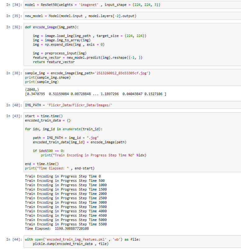
Images are nothing but input X to our model. Any input to a machine or deep learning model must be given in the form of numbers/vectors Hence all the images have to be converted into a fixed size vector which can then be fed as input to a Neural Network. For this purpose, transfer learning has been used. We will use a pre-trained model provided by keras library to interpret the content of the photos.

Transfer learning is a research problem in machine learning (ML) that focuses on storing knowledge gained while solving one problem and applying it to a different but related problem. For example, knowledge gained while learning to recognize cars could apply when trying to recognize trucks. Transfer learning is popular in deep learning given the enormous resources required to train deep learning models or the large and challenging datasets on which deep learning models are trained. In transfer learning, we can leverage knowledge (features, weights etc) from previously trained models for training newer models and even tackle problems like having less data for the newer task! Thus in this technique, we first train a base network on a base dataset and task, and then we repurpose the learned features, or transfer them, to a second target network to be trained on a target dataset and task. This process will tend to work if the features are general, meaning suitable to both base and target tasks, instead of specific to the base task.

When we train the network on a large dataset(for example: ImageNet) , we train all the parameters of the neural network and therefore the model is learned. It may take hours on your GPU. Convnet features are more generic in early layers and more base dataset specific in deeper layers.

We can give the new dataset to fine tune the pre-trained CNN. Consider that the new dataset is almost similar to the original dataset used for pre-training. Since the new dataset is similar, the same weights can be used for extracting the features from the new dataset.

When the new dataset is very small, it’s better to train only the final layers of the network to avoid overfitting, keeping all other layers fixed since they contain more generic features and thus we can get weights for our new data. So in this case we remove the final layers of the pre-trained network, add new layers and retrain only the new layers.

When the new dataset is very much large, we can retrain the whole network with initial weights from the pre-trained model.

Remark : How to fine tune if the new dataset is very different from the original dataset ?

Since, the earlier features of a ConvNet contain more generic features (e.g. edge detectors or color blob detectors), and later layers of the ConvNet becomes progressively more specific to the details of the classes contained in the original dataset. The earlier layers can help to extract the features of the new data. So it will be good if we fix the earlier layers and retrain the rest of the layers, if we have only small amount of data.

In this project, transfer learning has been used to extract features from images. The pre-trained model used is the ResNet model which is a model trained on ImageNet dataset .It has the power of classifying upto 1000 classes. ResNet model has skip connections which means the gradients can flow from one layer to another. This means the gradients can also backpropagate easily and hence ResNet model does not suffer from vanishing gradient problem. Figure shows the architecture of the model.

The whole ResNet model has not been trained from scratch. We are not interested in classifying images, but we are interested in the internal representation of the photo right before a classification is made. These are the “features” that the model has extracted from the photo. The Convolutional base is used as a feature extractor. After the convolutional base, a Global average pooling layer has been used to reduce the size of the activation map. Global Average Pooling takes a single channel at a time and averages all the values in that channel to convert it into a single value. The convolutional base produces an activation map of (7,7,2048). The Global Average Pooling layer takes the average of 7*7 (=49) pixels across all the 2048 channels and reduces the size of the activation map to (1,1,2048). So given an image, the model converts it into 2048 dimensional vector. Hence, we just remove the last softmax layer from the model and extract a 2048 length vector (bottleneck features) for every image. These feature vectors are generated for all the images of the training set and later will be sent to the final image captioning model to make predictions. We save all the train image features in a Python dictionary and save it on the disk using Pickle file, namely “encoded_train_img_features.pkl” whose keys are image names and values are corresponding 2048 length feature vector. Similarly we encode all the test images and save their 2048 length vectors on the disk to be used later while making predictions.

Note that

• The preprocess_input function converts images from RGB to BGR and then each color channel is zero-centered with respect to the ImageNet dataset, without scaling. Since we are using Transfer Learning, this is necessary so as to normalize our image data according to how it was trained in original ResNet-50 Model.
• “Pickling” is the process whereby a Python object hierarchy is converted into a byte stream, and “unpickling” is the inverse operation, whereby a byte stream (from a binary file or bytes-like object) is converted back into an object hierarchy.

The goal is to predict captions for different images. So during the training period, captions will be the target variables (Y) that the model is learning to predict. But the entire caption, given the image cannot be predicted all at once. Caption has to be predicted word by word. Thus each word has to be encoded into a fixed size vector. Since models work with numbers only, therefore to map each word in our vocabulary to some index, a python dictionary called word_to_idx has been created. Also the model outputs numbers which have to be decoded to form captions. Hence another python dictionary called idx_to_word to map each index with a word in the vocabulary has been created. These two Python dictionaries have been used as follows:

• word_to_idx[‘the’] -> returns index of the word ‘the’

• idx_to_word[10] -> returns the word whose index is 10

When the model is given a batch of sentences as input, the sentences maybe of different lengths. Hence to complete the 2D matrix or batch of sentences, zeros have been filled in for shorter sentences to make them equal in length to the longer sentences. The length of all the sentences have been fixed i.e equal to the length of the longest sentence in our vocabulary.

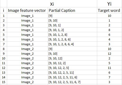
Now this can be framed as a supervised learning problem where we have a set of data points D = {Xi, Yi}, where Xi is the feature vector of data point ‘i’ and Yi is the corresponding target variable.

Image vector is the input and the caption is what we need to predict. But the way we predict the caption is as follows:

• In the first step we provide the image vector and the first word as input and try to predict the second word i.e. Input = Image_1 + ‘startseq’; Output = ‘the’
• Then we provide image vector and the first two words as input and try to predict the third word, i.e. Input = Image_1 + ‘startseq the’; Output = ‘cat’
• And so on…

Thus, each description will be split into words. The model will be provided one word and the photo and generate the next word. Then the first two words of the description will be provided to the model as input with the image to generate the next word. This is how the model will be trained.

It must be noted that, one image+caption is not a single data point but are multiple data points depending on the length of the caption. In every data point, it’s not just the image which goes as input to the system, but also, a partial caption which helps to predict the next word in the sequence.

However we cannot pass the actual English text of the caption, rather we pass the sequence of indices where each index represents a unique word. Since we had already created a dictionary word_to_idx, the data matrix after replacing the words with their indices is shown in figure below:

The model uses batch processing and due to that we need to make sure that each sequence is of equal length. Hence we need to append 0’s (zero padding) at the end of each sequence. For this we find out the maximum length, a caption has in the whole dataset. The maximum length of a caption in our dataset is 33. So we append those many number of zeros which will lead to every sequence having a length of 33. The data matrix will then look as shown

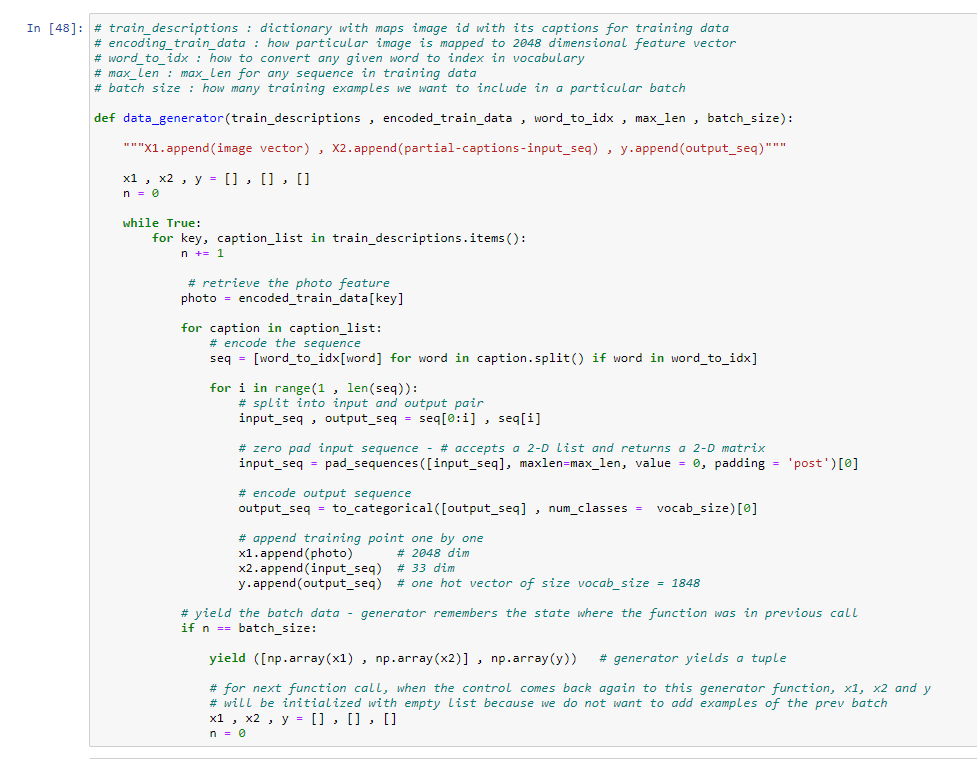
Now the question might arise that why do we need a Data Generator and can we use Keras inbuilt data generator or we have to create a Custom Data Generator ?

In our actual training dataset we have 6000 images, each having 5 captions. This makes a total of 30000 images and captions. Even if we assume that each caption on an average is just 7 words long, it will lead to a total of 30000*7 i.e. 210000 data points.

Size of the data matrix = n*m , where n -> number of data points (assumed as 210000) and m -> length of each data point

Clearly m = Length of image vector(2048) + Length of partial caption(x) = 2048 + x

x here is not equal to 33. This is because every word will be mapped to a higher dimensional space through some word embedding techniques. In this project , instead of training an embedding layer from scratch, Glove vectors have been used which is again an application of transfer learning. Glove vectors convert each word into a 50-dimensional vector. Since each partial caption contains 33 indices , where each index is a vector of length 50. Therefore, x = 33*50 = 1650. Hence m = 2048 + 1650 = 3698.

Finally the size of the data matrix = 210000 * 3698 = 776, 580, 000. Now even if we assume that 1 block takes 2 byte, then, to store this data matrix, we will require more than 3GB of main memory. This is a very huge requirement and will make the system very slow. For this reason we need a Custom Data Generator which is a functionality that is natively implemented in python. With SGD, we do not calculate the loss on the entire data set to update the gradients. Rather in every iteration, we calculate the loss on a batch of data points (typically 64, 128, 256, etc.) to update the gradients. This means that we do not require to store the entire dataset in the memory at once. Even if we have the current batch of points in the memory, it is sufficient for our purpose. We cannot use keras data generator because neither the directory structure nor the model layout is compatible with it.

A generator function in Python is used exactly for this purpose. It’s like an iterator which resumes the functionality from the point it left the last time it was called.

Word embedding is a technique used for the representation of words for text analysis, typically in the form of a real-valued vector that encodes the meaning of the word such that the words that are closer in the vector space are expected to be similar in meaning.

This section describes how indices of words of a caption have been converted into embeddings of fixed length. Whenever we feed data into RNN or LSTM layer, this data should have also been passed through the embedding layer. This embedding layer can be trained or we can pre - initialise this layer. In this project we have pre - initialised this layer by using Glove vectors from the file Glove6B50D.txt download Glove Vectors file from here. This txt file contains 50 dimensional word embeddings for 6 billion words. All 6 billion words are not needed and we just need the embeddings for the words that are there in our vocabulary.

Note : Words that are present in our vocab but are not there in the glove embeddings file will be substituted by all zeros(50-dimensional).

Image feature vector along with the partial sequence(caption) will be given to the model and the next word in the sequence is generated as the output. Then the output is again appended to the input and next word in the sequence is generated . This process continues until the model generates an ‘endseq’ token which marks the end of the caption. Figure shows the high level overview of the model architecture.

Since the input consists of two parts, an image vector and a partial caption, we cannot use the Sequential API provided by the Keras library. For this reason, we use the Functional API which allows us to create Merge Models.

Note : Since we have used a pre-trained embedding layer, we had to freeze it (trainable = False), before training the model, so that it does not get updated during the backpropagation.

We will describe the model in three parts:

Photo Feature Extractor - This is a ResNet-50 model pre-trained on the ImageNet dataset. We have pre-processed the photos with this model (without the output layer) and will use the extracted features predicted by this model as input.

Sequence Processor - This is a word embedding layer for handling the text input, followed by a Long Short-Term Memory (LSTM) recurrent neural network layer.

Decoder - Both the feature extractor and sequence processor output a fixed-length vector. These are merged together and processed by a Dense layer to make a final prediction.

The Photo Feature Extractor model expects input photo features to be a vector of 2,048 elements. These are processed by a Dense layer to produce a 256 element representation of the photo.

The Sequence Processor model expects input sequences with a pre-defined length (33 words) which are fed into an Embedding layer that uses a mask to ignore padded values. This is followed by an LSTM layer with 256 memory units.

Both the input models produce a 256 element vector. Now both the outputs are concatenated and sent to a MLP i.e. Multilayer Perceptron. Further, both input models use regularization in the form of 30% dropout. This is to reduce overfitting the training dataset, as this model configuration learns very fast.

The Decoder model merges the vectors from both input models using an addition operation. This is then fed to a Dense 256 neuron layer and then to a final output Dense layer which has nodes equal to the vocabulary size and thus, makes a probability prediction over the entire output vocabulary, using softmax activation function, for the next word in the sequence.

Since there are multiple outputs possible from the output layer, we have used categorical cross entropy as the loss function. The optimizer used to optimize the loss is the Adam optimizer.

Finally the weights of the model will be updated through backpropagation algorithm and the model will learn to output a word, given an image feature vector and a partial caption.