Outline

Questions
Warm Up
Load in Data
Conduct Hypothesis Testing

Objectives

YWBAT

conduct a 1 samp and 2 samp ttest using scipy.stats
test for criteria of 1 sample and 2 sample ttests

Warm Up

In a zoom chat, send an example of a type II error

What is a pvalue?

A probability that a data point would fall in to a set ASSUMING H0 IS TRUE.
The probability of an event occurring given the null hypothesis is true.
Pvalues change based on the problem
There is a debate on the validity of using Pvalues...

import pandas as pd
import numpy as np

import scipy.stats as scs
from sklearn.datasets import load_iris

import statsmodels.api as sm
import statsmodels.stats as stats

import matplotlib.pyplot as plt
import seaborn as sns

iris = load_iris()
data = iris.data
target = iris.target
features = iris.feature_names

df = pd.DataFrame(data, columns=features)
df['target'] = target
df.head()

.dataframe tbody tr th {
    vertical-align: top;
}

.dataframe thead th {
    text-align: right;
}

</style>

	sepal length (cm)	sepal width (cm)	petal length (cm)	petal width (cm)
0	5.1	3.5	1.4	0.2
1	4.9	3.0	1.4	0.2
2	4.7	3.2	1.3	0.2
3	4.6	3.1	1.5	0.2
4	5.0	3.6	1.4	0.2

df['target_names'] = df['target'].apply(lambda x: iris.target_names[x])

df.head()

.dataframe tbody tr th {
    vertical-align: top;
}

.dataframe thead th {
    text-align: right;
}

</style>

	sepal length (cm)	sepal width (cm)	petal length (cm)	petal width (cm)	target_names
0	5.1	3.5	1.4	0.2	setosa
1	4.9	3.0	1.4	0.2	setosa
2	4.7	3.2	1.3	0.2	setosa
3	4.6	3.1	1.5	0.2	setosa
4	5.0	3.6	1.4	0.2	setosa

df.target_names.unique()

array(['setosa', 'versicolor', 'virginica'], dtype=object)

print(iris.DESCR)

.. _iris_dataset:

Iris plants dataset
--------------------

**Data Set Characteristics:**

    :Number of Instances: 150 (50 in each of three classes)
    :Number of Attributes: 4 numeric, predictive attributes and the class
    :Attribute Information:
        - sepal length in cm
        - sepal width in cm
        - petal length in cm
        - petal width in cm
        - class:
                - Iris-Setosa
                - Iris-Versicolour
                - Iris-Virginica
                
    :Summary Statistics:

    ============== ==== ==== ======= ===== ====================
                    Min  Max   Mean    SD   Class Correlation
    ============== ==== ==== ======= ===== ====================
    sepal length:   4.3  7.9   5.84   0.83    0.7826
    sepal width:    2.0  4.4   3.05   0.43   -0.4194
    petal length:   1.0  6.9   3.76   1.76    0.9490  (high!)
    petal width:    0.1  2.5   1.20   0.76    0.9565  (high!)
    ============== ==== ==== ======= ===== ====================

    :Missing Attribute Values: None
    :Class Distribution: 33.3% for each of 3 classes.
    :Creator: R.A. Fisher
    :Donor: Michael Marshall (MARSHALL%[email protected])
    :Date: July, 1988

The famous Iris database, first used by Sir R.A. Fisher. The dataset is taken
from Fisher's paper. Note that it's the same as in R, but not as in the UCI
Machine Learning Repository, which has two wrong data points.

This is perhaps the best known database to be found in the
pattern recognition literature.  Fisher's paper is a classic in the field and
is referenced frequently to this day.  (See Duda & Hart, for example.)  The
data set contains 3 classes of 50 instances each, where each class refers to a
type of iris plant.  One class is linearly separable from the other 2; the
latter are NOT linearly separable from each other.

.. topic:: References

   - Fisher, R.A. "The use of multiple measurements in taxonomic problems"
     Annual Eugenics, 7, Part II, 179-188 (1936); also in "Contributions to
     Mathematical Statistics" (John Wiley, NY, 1950).
   - Duda, R.O., & Hart, P.E. (1973) Pattern Classification and Scene Analysis.
     (Q327.D83) John Wiley & Sons.  ISBN 0-471-22361-1.  See page 218.
   - Dasarathy, B.V. (1980) "Nosing Around the Neighborhood: A New System
     Structure and Classification Rule for Recognition in Partially Exposed
     Environments".  IEEE Transactions on Pattern Analysis and Machine
     Intelligence, Vol. PAMI-2, No. 1, 67-71.
   - Gates, G.W. (1972) "The Reduced Nearest Neighbor Rule".  IEEE Transactions
     on Information Theory, May 1972, 431-433.
   - See also: 1988 MLC Proceedings, 54-64.  Cheeseman et al"s AUTOCLASS II
     conceptual clustering system finds 3 classes in the data.
   - Many, many more ...

df.head()

.dataframe tbody tr th {
    vertical-align: top;
}

.dataframe thead th {
    text-align: right;
}

</style>

	sepal length (cm)	sepal width (cm)	petal length (cm)	petal width (cm)	target_names
0	5.1	3.5	1.4	0.2	setosa
1	4.9	3.0	1.4	0.2	setosa
2	4.7	3.2	1.3	0.2	setosa
3	4.6	3.1	1.5	0.2	setosa
4	5.0	3.6	1.4	0.2	setosa

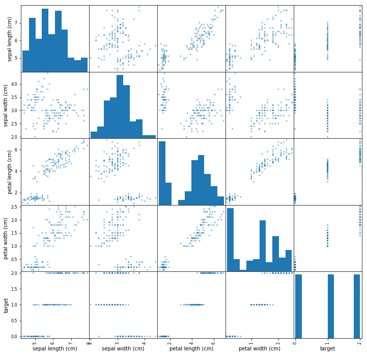
# pandas scattermatrix
pd.plotting.scatter_matrix(df, figsize=(12, 12))
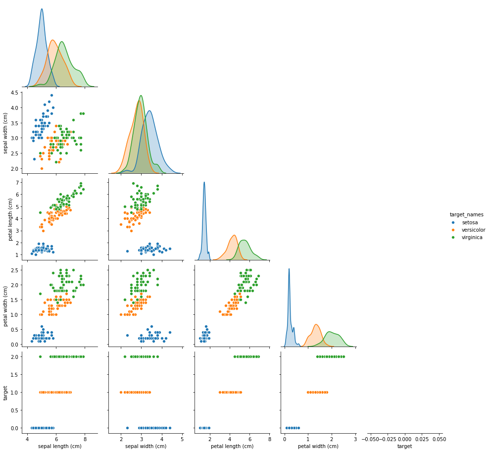
plt.show()

sns.pairplot(df, hue='target_names', corner=True)
plt.show()

/Users/rafael/anaconda3/envs/flatiron-env/lib/python3.6/site-packages/seaborn/distributions.py:288: UserWarning: Data must have variance to compute a kernel density estimate.
  warnings.warn(msg, UserWarning)

Q1. Is the mean sepal length different between virginica and versicolor iris flowers?

get data
ensure it's normal
take sampling statistics to compare the mean
run levene and shapiro tests
calculate cohen's d
write up findings

sl_virg = df.loc[df['target_names']=='virginica', 'sepal length (cm)']
sl_vers = df.loc[df['target_names']=='versicolor', 'sepal length (cm)']

what kind of test do we need to compare 2 populations?

2 sample ttest

what are the assumptions of a 2 sample ttest?

data is continuous - yes
data follows normal distribution - we need to test
variances are equal (otherwise you have to run a different ttest) - we need to test
independent - yes
sample things correctly and randomly - yes

what is the null and alternative hypothesis of a 2 sample ttest

H0: $\mu_\text{virginica} = \mu_\text{versicolor}$
HA: $\mu_\text{virginica} \neq \mu_\text{versicolor}$
H0: mu_virginica = mu_versicolor
HA: mu_virginica != mu_versicolor

step 1: test for normality

sl_virg.shape, sl_vers.shape

((50,), (50,))

# if i'm testing the means, I don't care about the populations
# what should I be taking
sample_mus_virginica = []
sample_mus_versicolor = []
for i in range(30):
    virgSamp = np.random.choice(sl_virg, size=50, replace=True).mean()
    versSamp = np.random.choice(sl_vers, size=50, replace=True).mean()
    sample_mus_virginica.append(virgSamp)
    sample_mus_versicolor.append(versSamp)

# test each sample for normality using shapiro
# h0: data was drawn from a normal distribution 
# ha: data was not drawn from a normal distribution
# if p<0.05 reject the null otherwise
# p >= 0.05 fail to reject the null
t1, p1 = scs.shapiro(sample_mus_virginica)
t2, p2 = scs.shapiro(sample_mus_versicolor)

print(p1)
print(p2)

# since p > 0.05 in both cases we fail to reject that the data is normal
# therefore we can assume that our data is normal

0.9824318289756775
0.935992419719696

# test for equal variances using a levene test
# h0: samples are from populations with equal variances
# ha: samples are not from populations with equal variances

t, p = scs.levene(sample_mus_virginica, sample_mus_versicolor)
p
# since p>0.05 we fail to reject that the variances are equal
# therefore we can assume that our variances are equal

0.33812261694131196

# Now that our assumptions are met we can actually do a ttest

# h0: mu_virginica = mu_versicolor
# ha: mu_virginica != mu_versicolor
t, p = scs.ttest_ind(sample_mus_virginica, sample_mus_versicolor, equal_var=False)
p

1.7437233880790833e-39

Initial Findings

After doing a sampling distribution of the mean and running a welch's ttest one can conclude that the mean sample length of each group is different.

Next Steps: Now let's measure how different these means are

# how do we measure difference of means? 
# power analysis

def cohen_d(x,y):
    nx = len(x)
    ny = len(y)
    dof = nx + ny - 2
    return np.abs(np.mean(x) - np.mean(y)) / np.sqrt(((nx-1)*np.std(x, ddof=1) ** 2 + (ny-1)*np.std(y, ddof=1) ** 2) / dof)

effect_size = cohen_d(sample_mus_virginica, sample_mus_versicolor)
effect_size

8.899510337442127

from statsmodels.stats.power import TTestIndPower

analysis = TTestIndPower()

result = analysis.solve_power(effect_size=effect_size, nobs1=30, alpha=0.05)
result

1.0

type2error_rate = 1 - result
type2error_rate

0.0

How do we interpret this?

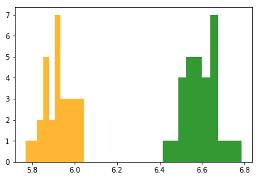
if you take a sample of versicolors or virginicas and measure the mean sepal length I can tell you with 100% certainity where the flowers came from.

plt.hist(sample_mus_virginica, color='green', alpha=0.8)
plt.hist(sample_mus_versicolor, color='orange', alpha=0.8)
plt.show()

Q2 Is the petal length different among any of the iris flowers (anova)

What did we learn today?

don't only eyeball normality
shapiro and levene test
pairplots are awesome and very useful for data viz
power analysis
- you'll always have 3 of 4 and it will always solve for the 4th
input into the scatter matrix
cohen's d to measure the effect size
alpha=0.05 because it's standard

Day 2 - ANOVA TESTING

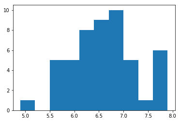
plt.hist(sl_virg)
plt.show()

sl_virg_zscores = scs.zscore(sl_virg)
random_zscores = np.random.normal(0, 1, 50)

# H0: sl_virg = normal distribution
# HA: sl_virg != normal distribution
scs.kstest(sl_virg_zscores, 'norm', args=(0, 1)) 

# pvalue of 0, which means we reject the null

KstestResult(statistic=0.11558941328638006, pvalue=0.48764984405744605)

random_normal_data = np.random.normal(50, 10, 1000)

# H0: random_normal_data = normal distribution
# HA: random_normal_data != normal distribution
scs.kstest(random_normal_data, 'norm', args=(50, 10))  
# pvalue of 0, which means we reject the null

KstestResult(statistic=0.03540056710981665, pvalue=0.15929441756654197)

def ks_test(arr):
    zscores_arr = scs.zscore(arr)
    t, p = scs.kstest(zscores_arr, 'norm', args=(0, 1))
    return t, p

ks_test(sl_virg)

(0.11558941328638006, 0.48764984405744605)

scs.anderson(sl_virg, 'norm')

AndersonResult(statistic=0.5516407106574732, critical_values=array([0.538, 0.613, 0.736, 0.858, 1.021]), significance_level=array([15. , 10. ,  5. ,  2.5,  1. ]))

In summary

Shapiro Wilks is less strict than a KS Test

use both

ANOVA Testing

When

Multiple Comparisons
Number of Ice Cream sold by Flavors
Sepal Length of all iris flowers (3)
Drug Testing (more than 2 groups)
Testing more than 2 groups

What does it tell you?

H0: u1 = u2 = ... = uN
HA: ui!=uj for some i and j in our groups

sl_seto = df.loc[df['target_names']=='setosa', 'sepal length (cm)']

step 1: take bootstrap sampling distributions

sl_sd_virg = []
sl_sd_vers = []
sl_sd_seto = []

for i in range(30):
    s1 = np.random.choice(sl_seto, 50, replace=True).mean()
    s2 = np.random.choice(sl_vers, 50, replace=True).mean()
    s3 = np.random.choice(sl_virg, 50, replace=True).mean()
    sl_sd_seto.append(s1)
    sl_sd_vers.append(s2)
    sl_sd_virg.append(s3)

step 2: test each sampling distribution for normality

for samp in [sl_sd_seto, sl_sd_vers, sl_sd_virg]:
    t, p = ks_test(samp)
    print(t, p)

# pvalues > 0.05 -> data is normal

0.07106849093676221 0.9981258672951128
0.10135268270444081 0.9175703455910869
0.1179278228199826 0.7983071102773645

step 3: test for equal variances

# H0: input samples are from equal variances
# HA: input samples are not from equal variances

scs.bartlett(sl_sd_seto, sl_sd_vers, sl_sd_virg)
# p<=0.05 -> reject the null variances are not equal the differenc of spreads isn't greater than 3

BartlettResult(statistic=17.335422788020647, pvalue=0.00017205241417272234)

step4: ANOVA test

# H0: u1 = ... = un
# HA: ui!=uj
scs.f_oneway(sl_sd_seto, sl_sd_vers, sl_sd_virg)

# p<0.05 reject the null

F_onewayResult(statistic=3518.8142885838843, pvalue=5.941971274788364e-84)

df['sl'] = df['sepal length (cm)']

import statsmodels.api as sm
from statsmodels.formula.api import ols

model = ols('sl ~ C(target_names)', data=df).fit()
anova_table = sm.stats.anova_lm(model, typ=2)
anova_table

.dataframe tbody tr th {
    vertical-align: top;
}

.dataframe thead th {
    text-align: right;
}

</style>

	sum_sq	df	F	PR(>F)
C(target_names)	63.212133	2.0	119.264502	1.669669e-31
Residual	38.956200	147.0	NaN	NaN

Conclusion

the sepal of at least one group is different than the another group

Comparing multiple groups

mc = stats.multicomp.MultiComparison(df['sepal length (cm)'], df['target_names'])

res = mc.tukeyhsd()
print(res)

   Multiple Comparison of Means - Tukey HSD, FWER=0.05   
=========================================================
  group1     group2   meandiff p-adj lower  upper  reject
---------------------------------------------------------
    setosa versicolor     0.93 0.001 0.6862 1.1738   True
    setosa  virginica    1.582 0.001 1.3382 1.8258   True
versicolor  virginica    0.652 0.001 0.4082 0.8958   True
---------------------------------------------------------

for col in df.columns[:4]:
    mc = stats.multicomp.MultiComparison(df[col], df['target_names'])
    print(f"Testing: {col}")
    res = mc.tukeyhsd()
    print(res)
    print("\n\n")

Testing: sepal length (cm)
   Multiple Comparison of Means - Tukey HSD, FWER=0.05   
=========================================================
  group1     group2   meandiff p-adj lower  upper  reject
---------------------------------------------------------
    setosa versicolor     0.93 0.001 0.6862 1.1738   True
    setosa  virginica    1.582 0.001 1.3382 1.8258   True
versicolor  virginica    0.652 0.001 0.4082 0.8958   True
---------------------------------------------------------



Testing: sepal width (cm)
    Multiple Comparison of Means - Tukey HSD, FWER=0.05     
============================================================
  group1     group2   meandiff p-adj   lower   upper  reject
------------------------------------------------------------
    setosa versicolor   -0.658  0.001 -0.8189 -0.4971   True
    setosa  virginica   -0.454  0.001 -0.6149 -0.2931   True
versicolor  virginica    0.204 0.0088  0.0431  0.3649   True
------------------------------------------------------------



Testing: petal length (cm)
   Multiple Comparison of Means - Tukey HSD, FWER=0.05   
=========================================================
  group1     group2   meandiff p-adj lower  upper  reject
---------------------------------------------------------
    setosa versicolor    2.798 0.001 2.5942 3.0018   True
    setosa  virginica     4.09 0.001 3.8862 4.2938   True
versicolor  virginica    1.292 0.001 1.0882 1.4958   True
---------------------------------------------------------



Testing: petal width (cm)
   Multiple Comparison of Means - Tukey HSD, FWER=0.05   
=========================================================
  group1     group2   meandiff p-adj lower  upper  reject
---------------------------------------------------------
    setosa versicolor     1.08 0.001 0.9831 1.1769   True
    setosa  virginica     1.78 0.001 1.6831 1.8769   True
versicolor  virginica      0.7 0.001 0.6031 0.7969   True
---------------------------------------------------------

Name		Name	Last commit message	Last commit date
Latest commit History 6 Commits
.ipynb_checkpoints		.ipynb_checkpoints
hypothesis-testing_files		hypothesis-testing_files
README.md		README.md
hypothesis-testing.ipynb		hypothesis-testing.ipynb

Provide feedback

Saved searches

Use saved searches to filter your results more quickly

Repository files navigation

Outline

Objectives

Warm Up

What is a pvalue?

Q1. Is the mean sepal length different between virginica and versicolor iris flowers?

what kind of test do we need to compare 2 populations?

what are the assumptions of a 2 sample ttest?

what is the null and alternative hypothesis of a 2 sample ttest

step 1: test for normality

Initial Findings

Next Steps: Now let's measure how different these means are

How do we interpret this?

Q2 Is the petal length different among any of the iris flowers (anova)

What did we learn today?

Day 2 - ANOVA TESTING

In summary

ANOVA Testing

step 1: take bootstrap sampling distributions

step 2: test each sampling distribution for normality

step 3: test for equal variances

step4: ANOVA test

Conclusion

Comparing multiple groups

About

Releases

Packages

Contributors 2

Languages

	sepal length (cm)	sepal width (cm)	petal length (cm)	petal width (cm)
0	5.1	3.5	1.4	0.2
1	4.9	3.0	1.4	0.2
2	4.7	3.2	1.3	0.2
3	4.6	3.1	1.5	0.2
4	5.0	3.6	1.4	0.2

	sepal length (cm)	sepal width (cm)	petal length (cm)	petal width (cm)
0	5.1	3.5	1.4	0.2
1	4.9	3.0	1.4	0.2
2	4.7	3.2	1.3	0.2
3	4.6	3.1	1.5	0.2
4	5.0	3.6	1.4	0.2

erdosn/hypothesis-testing-lesson

Folders and files

Latest commit

History

Repository files navigation

Outline

Objectives

Warm Up

What is a pvalue?

Q1. Is the mean sepal length different between virginica and versicolor iris flowers?

what kind of test do we need to compare 2 populations?

what are the assumptions of a 2 sample ttest?

what is the null and alternative hypothesis of a 2 sample ttest

step 1: test for normality

Initial Findings

Next Steps: Now let's measure how different these means are

How do we interpret this?

Q2 Is the petal length different among any of the iris flowers (anova)

What did we learn today?

Day 2 - ANOVA TESTING

In summary

ANOVA Testing

step 1: take bootstrap sampling distributions

step 2: test each sampling distribution for normality

step 3: test for equal variances

step4: ANOVA test

Conclusion

Comparing multiple groups

About

Resources

Stars

Watchers

Forks

Releases

Packages 0

Contributors 2

Languages

Packages

	sepal length (cm)	sepal width (cm)	petal length (cm)	petal width (cm)
0	5.1	3.5	1.4	0.2
1	4.9	3.0	1.4	0.2
2	4.7	3.2	1.3	0.2
3	4.6	3.1	1.5	0.2
4	5.0	3.6	1.4	0.2