NEW: The easiest way to get started using this code is probably by checking out the notebook tutorial.ipynb. This notebook is still work in progress, but contains basic functionality to define and train a planar flow, and visualise its output.

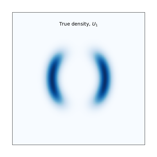
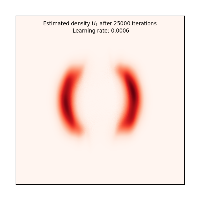
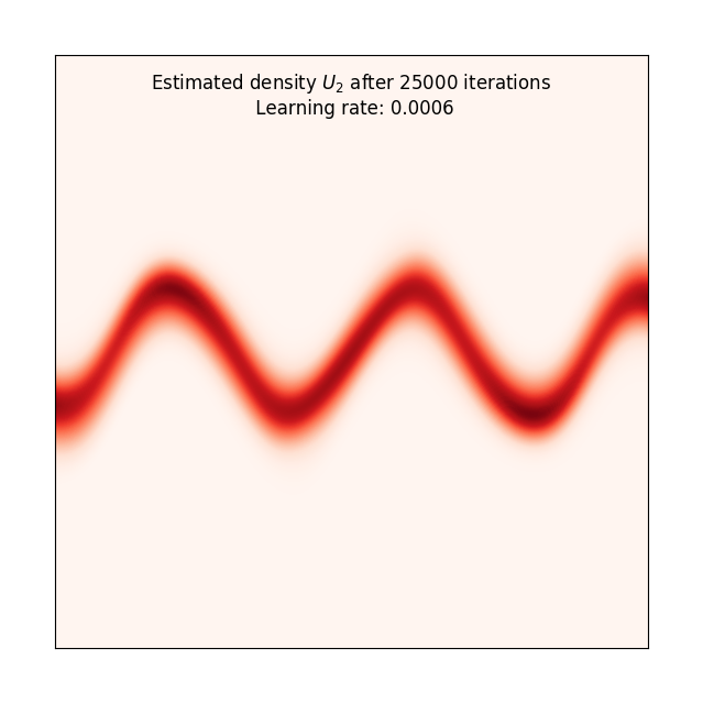
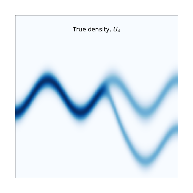
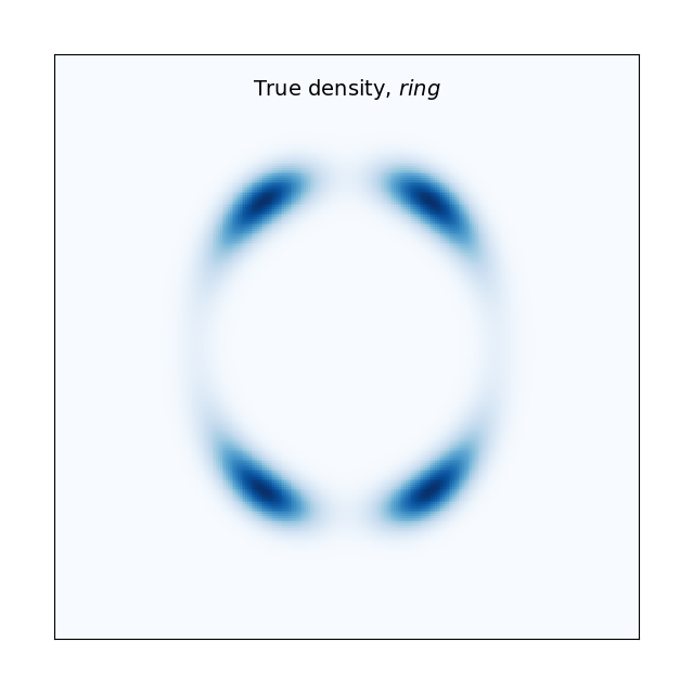
PyTorch implementation of planar flows as presented in the seminal paper "Variational inference with normalizing flows" by Danilo J. Rezende and Shakir Mohamed [1]. Below, I have replicated the results from Figure 3b in the paper. The flow length is set to K=32 for all experiments. The learning rate and number of iterations used are given by the captions for each plot. Set the hyperparameters of the normalising flow in train.py and run to reproduce these results. The potential functions to choose from are defined in target_distribution.py, and are named U_1,...,U_4,ring.

The experiments highlight the flexibility of normalising flows by showing that they can transform a standard Gaussian into multimodal and periodic densities. The animations are added to show how the normalising flow gradually expands and contracts the input space into the desired target density. By feeding samples from a standard bivariate Gaussian into the trained flow network, we can draw new samples from the target density. I have implemented the invertibility condition for planar flows from the appendix of [1], so we can also go the other way, i.e., estimate the likelihood of a point from the target density using the initial Gaussian density and the sum of the log-det-Jacobians of the transformations.

[1] https://arxiv.org/abs/1505.05770v6

True density	Estimated density	Animation