Pretty and opinionated topic model visualization in Python.

• Compatiblity with contextually sensitive topic models in Turftopic and BERTopic.
• Easier and more streamlined persistence and interoperability.
• Smaller building blocks for constructing figures and apps.

• Investigate complex relations between topics, words, documents and groups/genres/labels interactively
• Easy to use pipelines for classical topic models that can be utilized for downstream tasks
• Sklearn, Turftopic, Gensim and BERTopic compatible 🔩
• Interactive and composable Plotly figures
• Rename topics at will
• Share your results
• Easy deployment 🌍

Install from PyPI:

Notice that the package name on PyPI contains a dash: topic-wizard instead of topicwizard. I know it's a bit confusing, sorry for that

pip install topic-wizard

The main abstraction of topicwizard around a classical/bag-of-words models is a topic pipeline, which consists of a vectorizer, that turns texts into bag-of-words representations and a topic model which decomposes these representations into vectors of topic importance. topicwizard allows you to use both scikit-learn pipelines or its own TopicPipeline.

Let's build a pipeline. We will use scikit-learns CountVectorizer as our vectorizer component:

from sklearn.feature_extraction.text import CountVectorizer

vectorizer = CountVectorizer(min_df=5, max_df=0.8, stop_words="english")

The topic model I will use for this example is Non-negative Matrix Factorization as it is fast and usually finds good topics.

from sklearn.decomposition import NMF

model = NMF(n_components=10)

Then let's put this all together in a pipeline. You can either use sklearn Pipelines...

from sklearn.pipeline import make_pipeline

topic_pipeline = make_pipeline(vectorizer, model)

Or topicwizard's TopicPipeline

from topicwizard.pipeline import make_topic_pipeline

topic_pipeline = make_topic_pipeline(vectorizer, model)

You can also turn an already existing pipeline into a TopicPipeline.

from topicwizard.pipeline import TopicPipeline

topic_pipeline = TopicPipeline.from_pipeline(pipeline)

Let's load a corpus that we would like to analyze, in this example I will use 20newsgroups from sklearn.

from sklearn.datasets import fetch_20newsgroups

newsgroups = fetch_20newsgroups(subset="all")
corpus = newsgroups.data

# Sklearn gives the labels back as integers, we have to map them back to
# the actual textual label.
group_labels = [newsgroups.target_names[label] for label in newsgroups.target]

Then let's fit our pipeline to this data:

topic_pipeline.fit(corpus)

Models do not necessarily have to be fitted before visualizing, topicwizard fits the model automatically on the corpus if it isn't prefitted.

Then launch the topicwizard web app to interpret the model.

import topicwizard

topicwizard.visualize(corpus, model=topic_pipeline)

You can also use your gensim topic models in topicwizard by wrapping them in a TopicPipeline.

from gensim.corpora.dictionary import Dictionary
from gensim.models import LdaModel
from topicwizard.compatiblity import gensim_pipeline

texts: list[list[str] = [
    ['computer', 'time', 'graph'],
    ['survey', 'response', 'eps'],
    ['human', 'system', 'computer'],
    ...
]

dictionary = Dictionary(texts)
bow_corpus = [dictionary.doc2bow(text) for text in texts]
lda = LdaModel(bow_corpus, num_topics=10)

pipeline = gensim_pipeline(dictionary, model=lda)
# Then you can use the pipeline as usual
corpus = [" ".join(text) for text in texts]
topicwizard.visualize(corpus, model=pipeline)

topicwizard can also help you interpret topic models that understand contextual nuances in text, by utilizing representations from sentence transformers. The package is mainly designed to be compatible with turftopic, which to my knowledge contains the broadest range of contextually sensitive models, but we also provide compatibility with BERTopic.

Here's an example of interpreting a Semantic Signal Separation model over the same corpus.

import topicwizard
from turftopic import SemanticSignalSeparation

model = SemanticSignalSeparation(n_components=10)
topicwizard.visualize(corpus, model=model)

You can also use BERTopic models by wrapping them in a compatibility layer:

from bertopic import BERTopic
from topicwizard.compatibility import BERTopicWrapper

model = BERTopicWrapper(BERTopic(language="english"))
topicwizard.visualize(corpus, model=model)

The documentation also includes examples of how you can construct Top2Vec and CTM models in turftopic, or you can write your own wrapper quite easily if needed.

You can launch the topic wizard web application for interactively investigating your topic models. The app is also quite easy to deploy in case you want to create a client-facing interface.

import topicwizard

topicwizard.visualize(corpus, model=topic_pipeline)

From version 0.3.0 you can also disable pages you do not wish to display thereby sparing a lot of time for yourself:

# A large corpus takes a looong time to compute 2D projections for so
# so you can speed up preprocessing by disabling it alltogether.
topicwizard.visualize(corpus, pipeline=topic_pipeline, exclude_pages=["documents"])

Topics	Words

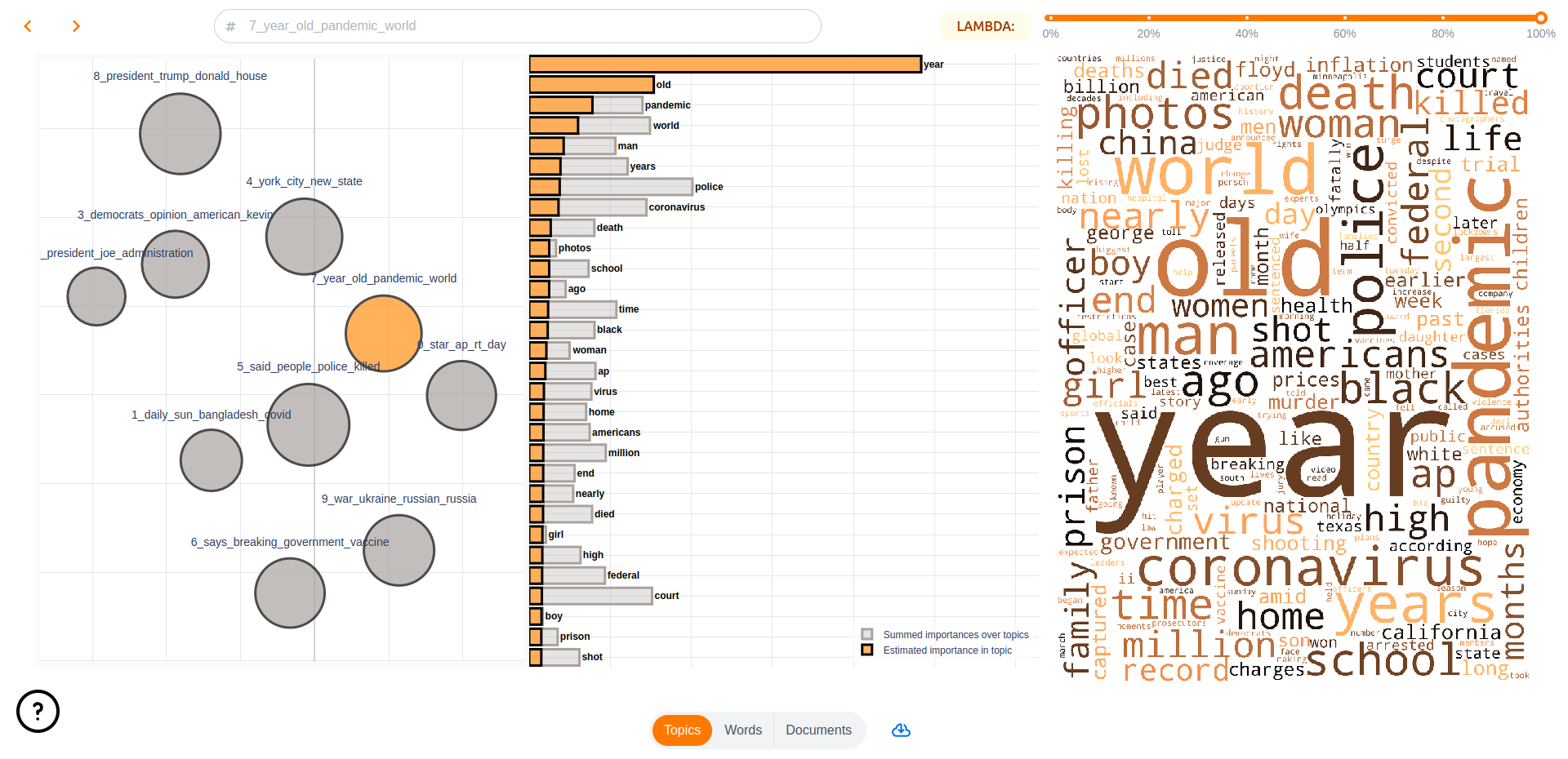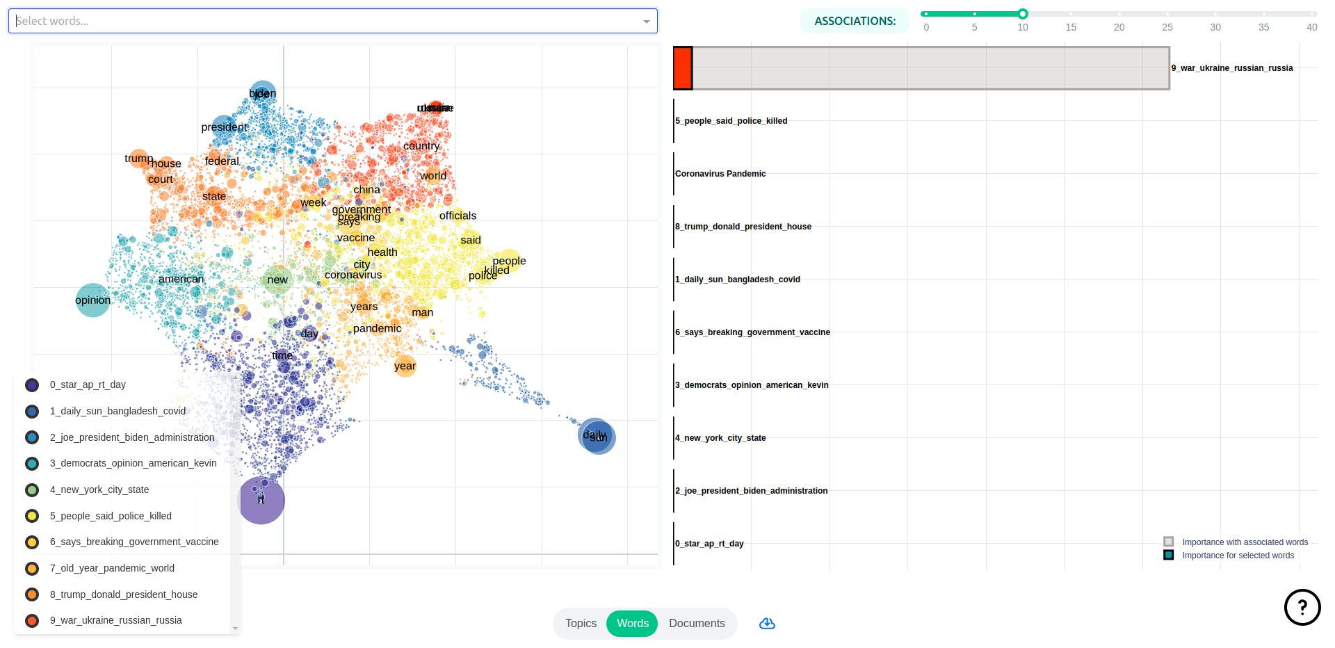Documents	Groups

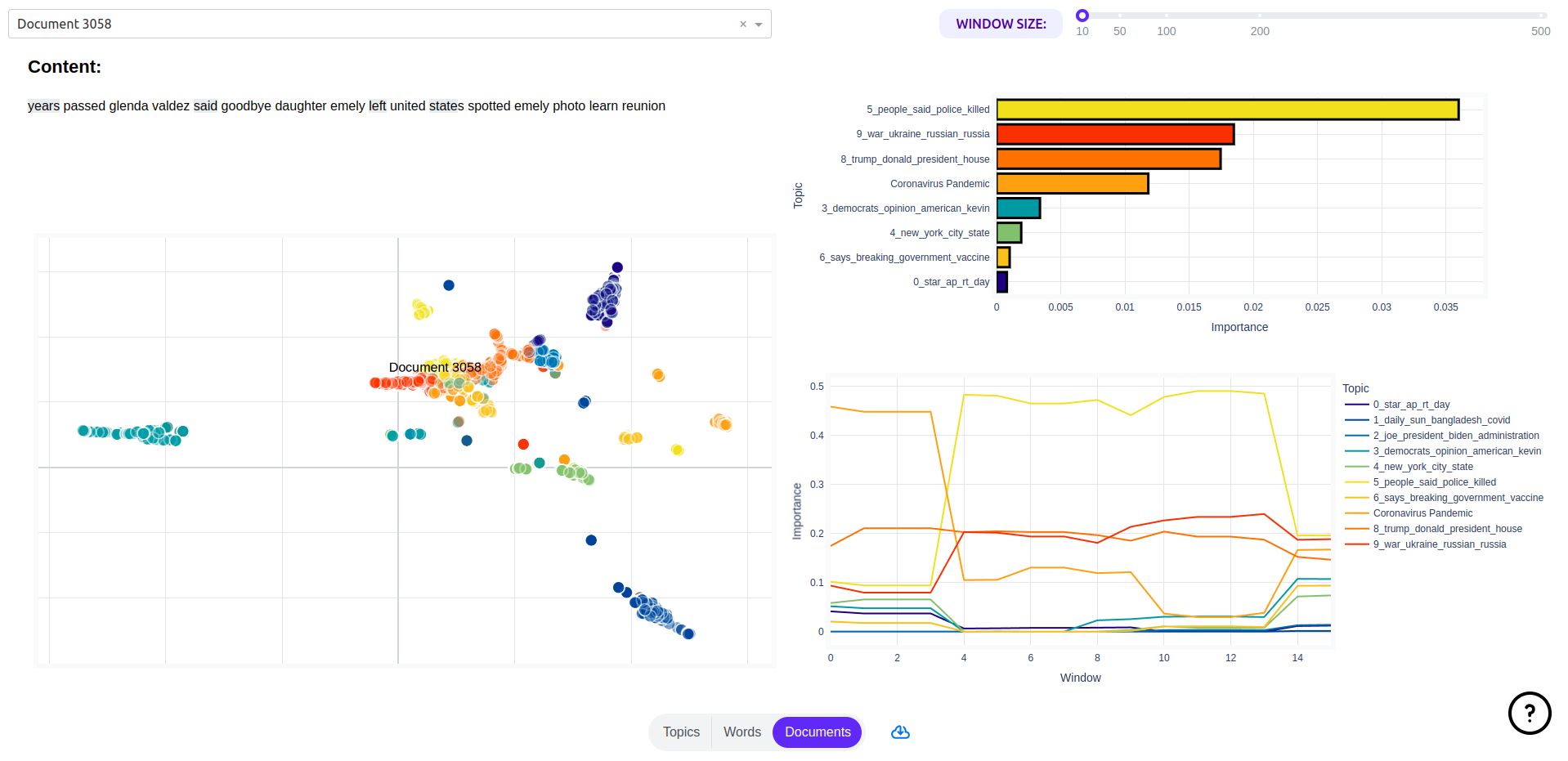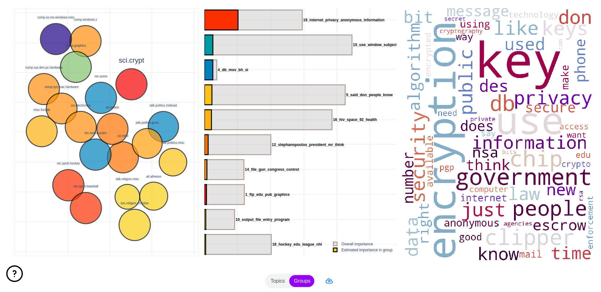All compatible models in topicwizard have a prepare_topic_data() method, which produces a TopicData object containing information about topical inference and model fit on a given corpus.

TopicData is in essence a typed dictionary, containing all information that is needed for interactive visualization in topicwizard.

You can produce this data with TopicPipeline

pipeline = make_topic_pipeline(CountVectorizer(), NMF(10))
topic_data = pipeline.prepare_topic_data(corpus)

And with contextual models:

model = SemanticSignalSeparation(10)
topic_data = model.prepare_topic_data(corpus)

# or with BERTopic
model = BERTopicWrapper(BERTopic())
topic_data = model.prepare_topic_data(corpus)

TopicData can then be used to spin up the web application.

import topicwizard

topicwizard.visualize(topic_data=topic_data)

This data structure can be serialized, saved and shared. topicwizard uses joblib for serializing the data.

Beware that topicwizard 1.0.0 is no longer fully backwards compatible with the old topic data files. No need to panic, you can either construct TopicData manually from the old data structures, or try to run the app anyway. It will probably work just fine, but certain functionality might be missing.

import joblib
from topicwizard.data import TopicData

# Save the data
joblib.dump(topic_data, "topic_data.joblib")

# Load the data
# (The type annotation is just for type checking, it doesn't do anything)
topic_data: TopicData = joblib.load("topic_data.joblib")

When sharing across machines, make sure that everyone is on the same page with versions of the different packages. For example if the inference machine has scikit-learn==1.2.0, it's advisable that you have a version on the server that is compatible, otherwise deserialization might fail. Same thing goes for BERTopic and turftopic of course.

In fact when you click the download button in the application this is exactly what happens in the background.

The reason that this is useful, is that you might want to have the results of an inference run on a server locally, or you might want to run inference on a different machine from the one that is used to deploy the application.

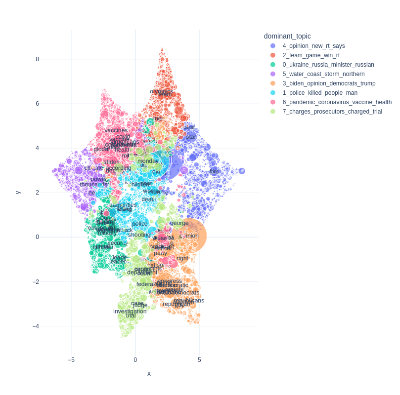
If you want customizable, faster, html-saveable interactive plots, you can use the figures API.

All figures are produced from a TopicData object so that you don't have to run inference twice on the same corpus for two different figures.

Here are a couple of examples:

from topicwizard.figures import word_map, document_topic_timeline, topic_wordclouds, word_association_barchart

Word Map	Timeline of Topics in a Document
word_map(topic_data)	document_topic_timeline(topic_data, "Joe Biden takes over presidential office from Donald Trump.")

Wordclouds of Topics	Topic for Word Importance
topic_wordclouds(topic_data)	word_association_barchart(topic_data, ["supreme", "court"])

Figures in topicwizard are in essence just Plotly interactive figures and they can be modified at will. Consult Plotly's documentation for more details about manipulating and building plots.

For more information consult our Documentation