The goals / steps of this project are the following:

• Perform a Histogram of Oriented Gradients (HOG) feature extraction on a labeled training set of images and train a classifier Linear SVM classifier
• Optionally, you can also apply a color transform and append binned color features, as well as histograms of color, to your HOG feature vector.
• Note: for those first two steps don't forget to normalize your features and randomize a selection for training and testing.
• Implement a sliding-window technique and use your trained classifier to search for vehicles in images.
• Run your pipeline on a video stream (start with the test_video.mp4 and later implement on full project_video.mp4) and create a heat map of recurring detections frame by frame to reject outliers and follow detected vehicles.
• Estimate a bounding box for vehicles detected.

Bellow is the final video generated by the pipeline

The scikit-image package has a built in function to extract Histogram of Oriented Gradient features. I use it to extract HOG features from images. Bellow are code lines:

# Define a function to return HOG features and visualization
def get_hog_features(img, orient, pix_per_cell, cell_per_block,
                     vis=False, feature_vec=True):
    # Call with two outputs if vis==True
    if vis == True:
        features, hog_image = hog(img, orientations=orient,
                                  pixels_per_cell=(pix_per_cell, pix_per_cell),
                                  cells_per_block=(cell_per_block, cell_per_block),
                                  transform_sqrt=True,
                                  visualise=vis, feature_vector=feature_vec)
        return features, hog_image
    # Otherwise call with one output
    else:
        features = hog(img, orientations=orient,
                       pixels_per_cell=(pix_per_cell, pix_per_cell),
                       cells_per_block=(cell_per_block, cell_per_block),
                       transform_sqrt=True,
                       visualise=vis, feature_vector=feature_vec)
        return features

In this project, I put majority of the functions in one separate python file, "lesson_functions.py".

I then explored different color spaces and different skimage.hog() parameters (orientations, pixels_per_cell, and cells_per_block).
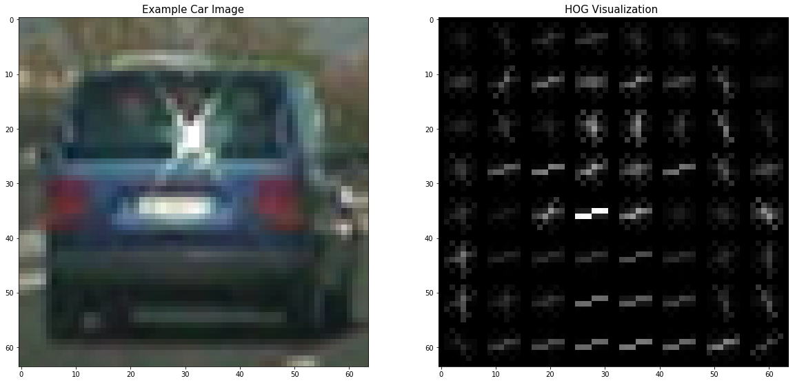
I grabbed random images from each of the two classes and displayed them to get a feel for what the skimage.hog() output looks like.

Here is an example using the YCrCb color space and HOG parameters of orientations=8, pixels_per_cell=(8, 8) and cells_per_block=(2, 2):

I started to use the parameters in class, and then tried various combinations of parameters. It is little empirical in my case, I tuned based on the final classification accuracy by various of tryings. Finally tried following values as parameters in my final video:

color_space = 'YCrCb' # Can be RGB, HSV, LUV, HLS, YUV, YCrCb
spatial_size = (16, 16)
hist_bins = 32
orient = 11
pix_per_cell = 8
cell_per_block = 2
hog_channel = 'ALL'
spatial_feat = True
hist_feat = false
hog_feat = True

I created a linear SVM using

svc = LinearSVC(C=0.01, loss='squared_hinge', penalty='l2', dual=True)

Then load training data and verify with the test data. Data are come from "vehicles" and "non-vehicles" downloads. Please check the project README to find out the download link.

Here we use a customized C = 0.01, a lower C value should help with any over-fitting of the training data.

After load the images, randomly shuffle the data, and split data to two groups with 20-80 ratio, 80% for training, and the other 20% for verification. Bellow are the code lines used to split data

rand_state = np.random.randint(0, 100)
X_train, X_test, y_train, y_test = train_test_split(
    scaled_X, y, test_size=0.2, random_state=rand_state)

Bellow is the training and verification results, with a accuracy = 98.73%.

Using: 11 orientations 8 pixels per cell and 2 cells per block
Feature vector length: 7332
19.71 Seconds to train SVC...
Test Accuracy of SVC =  0.9827

To minimize the window numbers (for performance concern), the scale algorithm I used is following bellow steps:

1. start at the middle of image, at the top center of the interest area (the area we used in Lane detection)
2. start with a small window width and height, and overlap value
3. Then expand the window with around %80 in next scale, iterate to step 2#

Bellow is my algorithm:

    for scale in range(1, 4):
        windowWidth = endx - startx

        startx = np.int(startx - windowWidth * 0.3)
        endx = np.int(endx + windowWidth * 0.3)

        windowHeight = np.int(endy - starty)
        starty = np.int(starty - windowHeight * 0.3)
        endy = np.int(endy + windowHeight * 0.3)

    #if (startx > x_start_stop[0] + (img.shape[1] - starty) - windowWidth) and (endx < x_start_stop[1]):
    window_list.append(((startx, starty), (endx, endy)))

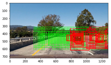
At the same time, also setup some start and stop X and Y, to minimize the area which used to scan the sliding windows. Bellow is one sample out put the of the sliding window: Here I found that using a ratio = 0.3 when expands the width and height can get best results. I use ratio = 0.4 at the beginning which draw the rectagle at the front of the drive way, which will cause unnecessary brake.

Also add one more step to the final pipeline, use Deque to cache latest 5 frames' hot windows, then increase the heatmap threshold, this help to avoid false positive too.

Follow are code lines about this algorithms:

from collections import deque
hotWindowsDeque = deque(maxlen = 5)

hot_windows = search_windows(draw_image, windows, svc, X_scaler, color_space=color_space, 
                        spatial_size=spatial_size, hist_bins=hist_bins, 
                        orient=orient, pix_per_cell=pix_per_cell, 
                        cell_per_block=cell_per_block, 
                        hog_channel=hog_channel, spatial_feat=spatial_feat, 
                        hist_feat=hist_feat, hog_feat=hog_feat)                       

hotWindowsDeque.append(hot_windows)

heat = np.zeros_like(draw_image[:,:,0]).astype(np.float)


# Add heat to each box in box list
for hw in hotWindowsDeque:
    heat = add_heat(heat,hot_windows)

# Apply threshold to help remove false positives
heat = apply_threshold(heat,threshold)

Ultimately I searched on 4 scales using HLS All channel HOG features plus spatially binned color and histograms of color in the feature vector, which provided a nice result.

When I use classifier predict the images, I check the confidence first, only results above some threshold will be treated as positive. This help reduce the false positive.

Following are some lines (in lesson_functions.py l284-288)

    # 6) Predict using your classifier
    prediction = clf.predict(test_features)

    confidence = clf.decision_function(test_features)

    # 7) If positive (prediction == 1) then save the window
    if prediction == 1 and abs(confidence) > 0.4:
        on_windows.append(window)

Here are some example images which show the vehicles detected:

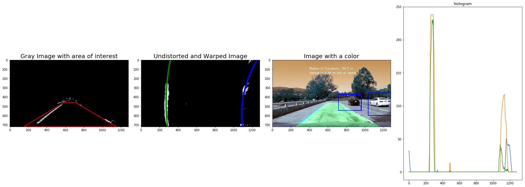
After added the "Vehicle Detection" step into the lane detection pipeline, bellow is one sample of the output of some steps:

Here's a link to my video result

Other versions of videos got during my steps of tuning. V1 V2 V3 V4 V5

Describe how (and identify where in your code) you implemented some kind of filter for false positives and some method for combining overlapping bounding boxes.

I recorded the positions of positive detections in each frame of the video. From the positive detections I created a heatmap and then thresholded that map to identify vehicle positions.
I then used scipy.ndimage.measurements.label() to identify individual blobs in the heatmap. I then assumed each blob corresponded to a vehicle. I constructed bounding boxes to cover the area of each blob detected.

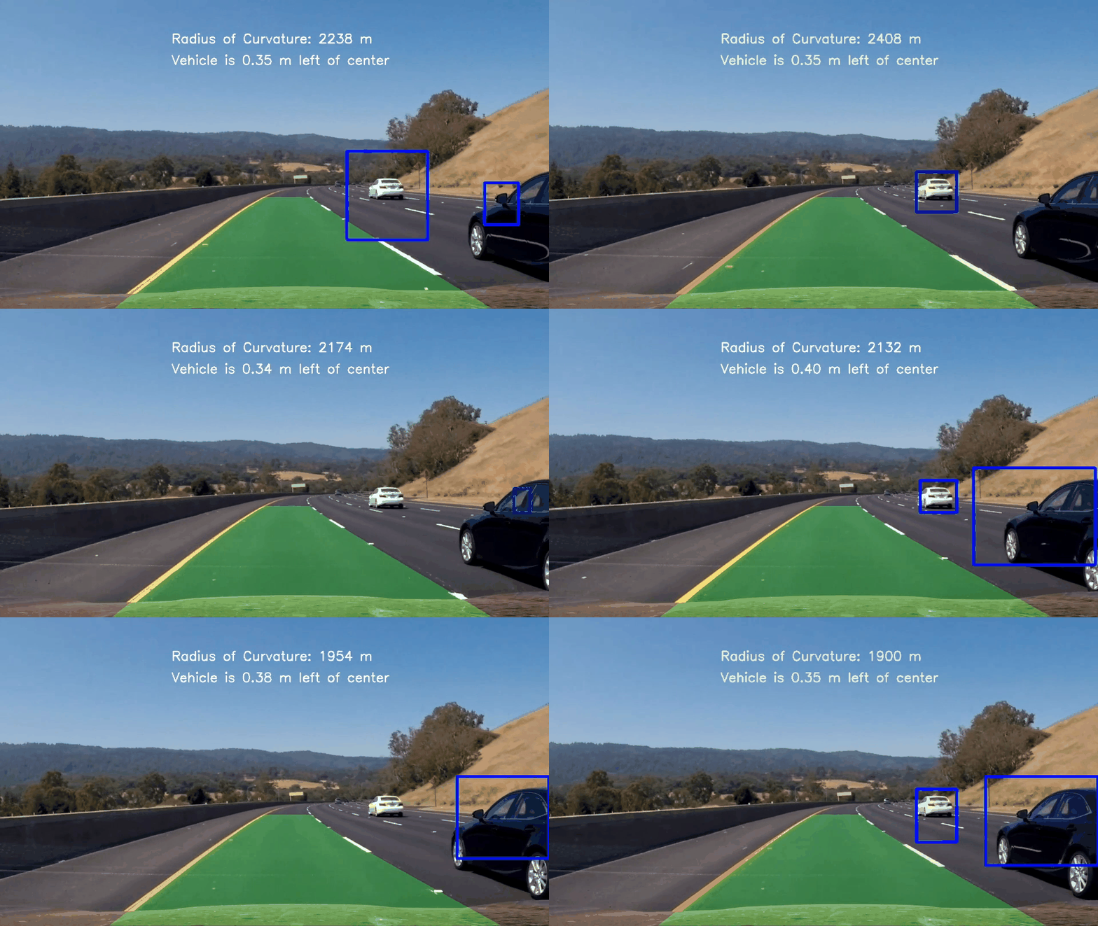
Here are six samples and their corresponding sliding windows, heatmaps and final rectangle bounding boxes:

Here I'll talk about the approach I took, what techniques I used, what worked and why, where the pipeline might fail and how I might improve it if I were going to pursue this project further.

1. Overall this project basically links all what I learn in this term1, including lane detection, image classification (here we use linear SVM instead of the deep learning algorithm), and lot of image processing algorithms.
2. Since this project is focusing on learning, I explicitly setup each step in the pipeline, and plot images in the middle of each step, which do help me understanding how the algorithm works. Some of the steps can be simplified, and merge, but in this project I did not.
3. Also known there are so many parameters in each step which need to be tuned. Some of them can be start by randomly settings, then the algorithms will automatically tune it (like in the deep learning session, all starting weights can be random). ). But some of the parameters need empirical configurations, or use some dedicated API to do permutation combination, then manually pick the the optimized ones. Parameter tuning is very key of the final pipeline, and determine the quality of the final delivery.
4. Another thing need to take care is the length of the pipeline, and the cost of each step. When more and more steps added, long pipeline will be a burden of the performance. In this project, since I merge all the steps from advanced lane detection with the new steps of HOG, sliding windows, car-noncar prediction, heatmap, labels, which make the pipeline very slow. As next step, need to look deeper, may need to simplify or merge some steps, or cache some middle compute results.
5. To make more professional code, need to maintain some own libraries and share them across the steps of the pipeline; also need a better framework which can load data, report data and give easy way to visualize the data for both middle outputs and final outputs. For Self-Driving car, to create a dedicated software platform are a must have.
6. For classification, training data are key, and augmentation the training data and make sure they are balance are the key of the key. This will help prevent potential over-fitting in majority of cases.
7. Finally but not least, understand and know how to use image processing algorithms are very important in self-pilot car implementation.