Title: Development of an algorithm for automatic detection of meniscus tears in knee magnetic resonance imaging (MRI) scans.
Utilising machine learning models as a computational technique for the diagnosis of osteoarthritis is still relatively new. The aim in this project is to develop a machine learning algorithm, and as proof of concept, to determine if the algorithm can identify meniscus tears by differentiating/ localizing abnormalities in MRI scans of the knee.
Osteoarthritis (OA) is the most prevalent medically treated arthritic condition worldwide. Diagnosis of symptomatic OA is usually made on the basis of clinical examination/ radiography and reported pain in the same joint. A meniscal tear is a frequent orthopaedic diagnosis and an early indication of OA. However, 61% of randomly selected subjects who showed meniscal tears in their knees during magnetic resonance imaging (MRI) scans, have not had any pain, aches, or stiffness during the previous months (Englund et al., 2008). So, meniscal tears are frequently encountered in both asymptomatic and symptomatic knees (Zanetti et al., 2003). Since an early detection of meniscal tear in asymptomatic knee appears to be an early indicator of OA and a risk factor for other articular structural changes, there is a need for a better and faster identification of meniscal tears (Ding et al., 2007). This is especially important in the absence of specialised radiologists, or a backlog due to increased use of medical imaging (McDonald et al., 2015, Kumamaru et al., 2018).
Data is from MRNet. It consists of 1370 knee MRI exams performed at Stanford University Medical Center. The dataset contains 1,104 (80.6%) abnormal exams, with 319 (23.3%) ACL tears and 508 (37.1%) meniscal tears; labels were obtained through manual extraction from clinical reports. The original dataset is 5D tensor with shape (batch_shape, s, conv_dim1, conv_dim2, channel), where s is the number of slices per scan. The training set consists of 1130 MRI images from coronal, sagittal and axial planes. The validation set consists of 120 images from coronal, sagittal and axial planes.
Metrics were accuracy and precision. Accuracy was used to determine the overall performance of the model.
MRI scanning is costly and requires a long scanning time. A patient would only be sent for an MRI scan, if further imaging evaluation is required. Thus, precision was used as another metric since I need to know how many of the positives were true positives. Due to time and costs, the more false positives there are, the more costly each true positive is.
| notebook | model | dataset | diagnosis |
|---|---|---|---|
| meniscus_resnet50 | resnet50 | extracted three | meniscus |
| meniscus_vgg16 | vgg16 | extracted three | meniscus |
| meniscus_alexnet | alexnet | extracted three | meniscus |
| meniscus_ownmodel | own | extracted one | meniscus |
| kneeone_ownmodel | own | extracted one | meniscus, acl, abnormal |
| meniscus_fulldata | own | full data | meniscus |
| meniscus_functional | functional | extracted one | meniscus |
Transfer learning is a research problem in machine learning (ML) that focuses on storing knowledge gained while solving one problem and applying it to a different but related problem. For example, knowledge gained while learning to recognize cars could be applied when trying to recognize trucks (source).
In this project, I will discuss Resnet50 & VGG16. Keras offers many other models.

ResNet-50 is a convolutional neural network that is 50 layers deep. It was first introduced in 2015 (He et al., 2015), and become really popular after winning several classification competitions. Since it is FIFTY layers deep, the stacked layers can enrich the features of the models, and work well with unstructured data.
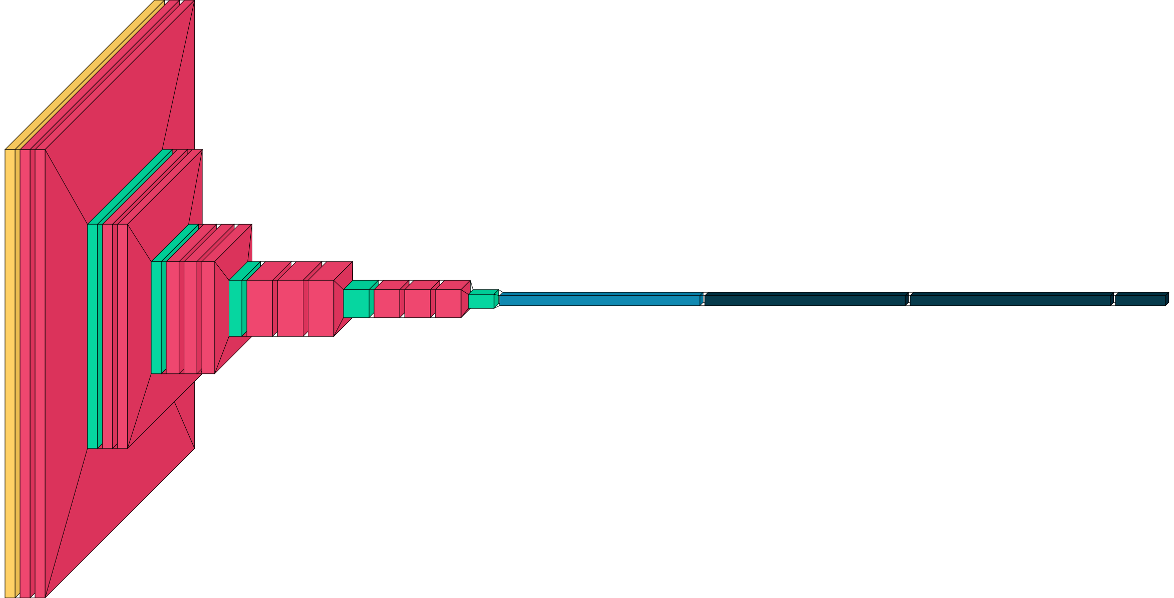
Unfortunately, when using a pretrained model, one is limited by input_shape. For ResNet50, it should be in 4D tensor with shape (batch_shape, conv_dim1, conv_dim2, channel). Thus, middle three images were extracted from each MRI scan, and used as inputs into the model. Only the last convolutional block of ResNet and added fully-connected layers were trained. Other layers were frozen. Due to the complexity of the model, there was a tendency to overfit. Tuning of kernel_regularizer and dropout parameters were used to minimise overfitting. EarlyStopping and ModelCheckpoint were used to monitor validation loss, and training was stopped if there was no changes to validation loss. Despite best attempts, the average validation accuracy is 0.567. While deep layers can provide better self-learning capabilities, it can also lead to degradation (ie, the accuracy layers may saturate and then slowly degrade after a point). Thus, model performance might deteriorate on both training and testing sets. To that end, due to the deep layers, the ResNet50 model was considered too complex for the dataset.

The VGG model was created by Oxford Visual Geometry Group (VGG), which helped fueled transfer learning work on new predictive modeling tasks. Despite winning the ImageNet challenge in 2014, the VGG models (VGG16, VGG19) are no longer considered state-of-the-art. However, they are still powerful pre-trained models that are useful as the basis to build better predictive image classifiers, and a good foundation for this project.
Similarly to ResNet, the input shape for VGG16 should be in 4D tensor with shape (batch_shape, conv_dim1, conv_dim2, channel). Thus, middle three images were extracted from each MRI scan, and used as inputs into the model. Only the last convolutional block of VGG16 and added fully-connected layers were trained. Other layers were frozen. Despite having only 23 layers, there was a tendency to overfit. Kernel_regularizer, batch normalisation and dropout were tuned to minimise overfitting. However, a GlobalAveragePooling layer with a Dropout of 0.6 worked well to minimise overfitting. Despite this, mean accuracy remains poor, at 0.56 for all three planes. Mean precision was 0.45. Due to the tendency to overfit, VGG16 was also considered too complex for the dataset.
Since the pretrained models were too complex for the dataset, demonstrated a tendency to overfit, and I am limited by what I can do to improve the dataset, I decided to build my own models instead. The models should be relatively 'simplier' than the previous pretrained models. There are, however, several challenges in building a model from scratch. Firstly, 1130 is too small a dataset for training. Secondly, a self-built model would usually result in a lower performance.

The model is adapted from AlexNet which won the 2012 ImageNet LSVRC-2012 competition, and which was also the primary building block for the Stanford group that analysed this data. It is not a pretrained model, and none of the layers were frozen. It is a lot 'smaller', with reduced number of filters and neurons in the connected layers to minimise overfitting. Similarly to previous models, middle three images were extracted from each MRI scan, and used as inputs into the model. 'same' padding was added, so that output size is the same as input size; This requires the filter window to slip outside input map, hence the need to pad.
To minimise overfitting, kernel_regularization, batch normalisation and dropout were tuned. Accuracy scores were found to fluctuate heavily over 50%, which implies that the model is not better than flipping a coin. So to ensure that the model is learning, and increasing its ability to generalise, smaller batch sizes of 8, 16, 32, and 64 were tested. Too small a batch size, and the model loses its ability to generalise, since there is too much noise, and learning is volatile. Too large a batch size, and the model also loses its ability to generalise, and the learning is slower. However, there is a higher chance that convergence to a global optima might occur. Batch size of 32 was chosen in the end. In addition, sgd's learning rate was decreased to 1e-5. Importantly, lowering the learning rate and decreasing the batch size actually allows the model to train better. Nevertheless, mean accuracy was at 0.575 for all three planes; Mean precision was 0.57.

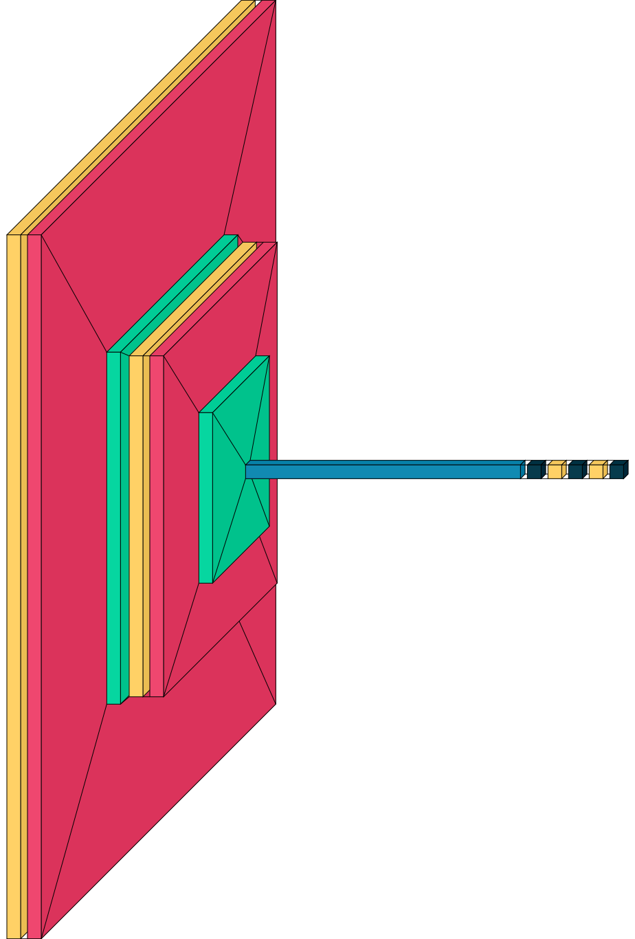
This model is a simple stack of two convolution layers with a ReLU activation and followed by max-pooling layers. This is very similar to the architectures that Yann LeCun built in the 1990s for image classification (with the exception of ReLU) (LeCun et al., 1998). In addition, three fully-connected layers were added, which ends with a single unit and a sigmoid activation, for a binary classification. I made LeNet even smaller by reducing the number of neurons in the connected layers.
To minimise overfitting, kernel_regularization, batch normalisation and dropout were tuned. To actually control the learning rate of the optimser, sgd with a slow learning rate and momentum were selected based on previous experience with AlexNet. Geometric mean of the accuracy of the three models was 0.575, and mean precision was 0.667.
Stacked classifier
Predictions from each model (of each plane) was combined/stacked and become new features for training another classifier to compute the final prediction. This acts as a stacked generalization where the outputs of the models were used an inputs into another classifier. Logistic regression model was used since each plane would be given the best weight. The plane with the highest weightage is the axial plane, followed by the coronal plane, and then the sagittal plane. Accuracy increased to 0.60, but precision decreased to 0.41.

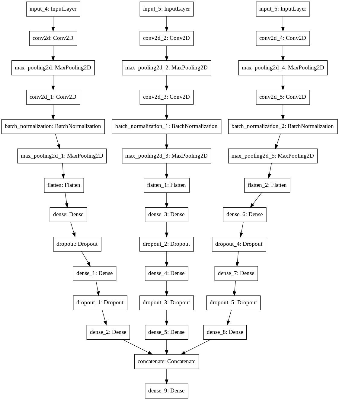
The Keras functional API was explored, since it can handle models with multiple inputs. Three inputs (one from each plane) was used for three parallel models, leading to one output. To minimise overfitting, kernel_regularization, batch normalisation and dropout were tuned. Batch size and sgd's learning rate were also explored. Unlike the stacked classifier with logistic regression, each plane was assumed to have equal weightage. Accuracy was similar to the geometric mean of previous models at 0.575. However, precision significantly increased to 1.0.