This package implements the Synthetic Difference-in-Differences method described by Arkhangelsky et al. (2021), who provide an implementation in R, with accompanying materials here: synthdid. We follow the implementation provided by Clarke et al. (2023) for Stata and adapt it for the Julia programming language.

The latest version can be downloaded and installed by running:

import Pkg; Pkg.add(url = "https://github.com/d2cml-ai/Synthdid.jl")

The latest stable version can be downloaded from Registry by running:

import Pkg; Pkg.add("Synthdid")

using Synthdid, DataFrames

The main function in Synthdid is the SynthDID constructor for the object type of the same name.

• data: DataFrame with the necessary data for the estimation. It must contain panel data for an outcome column, a column with the names or IDs of the units in the sample, a time column, and a column with an indicator for the periods in which each unit has been treated.
• Y_col: String or Symbol for the outcome variable
• S_col: String or Symbol for the unit variable
• T_col: String or Symbol for the time variable
• D_col: String or Symbol for the treatment variable
• covariates: Vector with column names for covariates
• cov_method: Either "projected" or "optimized". Choose how the residuals for estimation are calculated when adding covariates

This implementation is identical to the one presented by Arkhangelsky et al.

data = california_prop99();

res = sdid(data, :PacksPerCapita, :State, :Year, :treated);
res["att"]

-15.603827872733849

In the case of staggered treatments, the treated sample is separated by adoption year and several ATT are calculated with each partial sample and all the controls. The final ATT is the average of the partial ATTs weighted by the total amount of treatment years its subsample contains.

data = quota();

res = sdid(data, :womparl, :country, :year, :quota);
res["att"]

8.034101989321492

This method also stores each subsample's result, as well as relevant information and data for each iteration of the Synthetic Difference-in-Differences algorithm:

res["year_params"]

7×7 DataFrame
 Row │ treat_year  tau        weighted_tau  N0     T0    N1   T1
     │ Any         Any        Any           Any    Any   Any  Any
─────┼─────────────────────────────────────────────────────────────
   1 │ 2000.0      8.38887    1.42789       110.0  10.0  1.0  16.0
   2 │ 2002.0      6.96775    2.0755        110.0  12.0  2.0  14.0
   3 │ 2003.0      13.9523    3.85913       110.0  13.0  2.0  13.0
   4 │ 2005.0      -3.45054   -0.403787     110.0  15.0  1.0  11.0
   5 │ 2010.0      2.74904    0.17547       110.0  20.0  1.0  6.0
   6 │ 2012.0      21.7627    0.926073      110.0  22.0  1.0  4.0
   7 │ 2013.0      -0.820324  -0.0261805    110.0  23.0  1.0  3.0

There are two methods for adjusting for covariates in the estimation. The first one is proposed by Arkhangelsky et al. (2021), and it adjusts the outcome by the covariates in each subsample. As a result, this method is fairly slow as the procedure repeats for every subsample. This method is the package's default and can be called using the cov_method = "optimized" option:

data = dropmissing(data, :lngdp);
res = sdid(data, :womparl, :country, :year, :quota, covariates = [:lngdp], cov_method = "optimized")
res["att"]

8.047948491131669

The second method is proposed by Kranz (2022), for a faster adjustment of the outcome variable, as the procedure is only excecuted once for the whole sample. This method can be called using the cov_method = "projected" option:

res = sdid(data, :womparl, :country, :year, :quota, covariates = [:lngdp], cov_method = "projected")
res["att"]

8.059034614789997

We implement three methods for standard error: jackknife_se, bootstrap_se y placebo_se. Details about the implementation can be found at Clarke et al. (2023)

placebo_se(data, :womparl, :country, :year, :quota, covariates = [:lngdp], cov_method = "projected")

Placebo replications (50). This may take some time.
----+--- 1 ---+--- 2 ---+--- 3 ---+--- 4 ---+--- 5
..................................................     50

1.8918455360543351

For convenience, all the procedures described above can be executed and their results can be sumarized by using the SynthDID constructor and type.

res = SynthDID(data, :womparl, :country, :year, :quota, covariates = [:lngdp], cov_method = "projected");
res

Placebo replications (50). This may take some time.
----+--- 1 ---+--- 2 ---+--- 3 ---+--- 4 ---+--- 5
..................................................     50

1×6 DataFrame
 Row │ ATT      Std. Err.  t        P>|t|       [95% Conf.  Interval]
     │ Float64  Float64    Float64  Float64     Float64     Float64
─────┼────────────────────────────────────────────────────────────────
   1 │ 8.05903    1.65142  4.88005  1.06058e-6     4.82224    11.2958

This package uses the GR backend for Plotly, which allows to quickly generate plots and save them in png, pdf, ps, or svg format. All plots are stored in a dictionary by treatment year subsample.

We implement plotting outcome variable comparations:

plots = plot_outcomes(data, :PacksPerCapita, :State, :Year, :treated)
plots["1989"]

Plotting weights is also implemented:

plots = plot_weights(data, :PacksPerCapita, :State, :Year, :treated)
plots["1989"]

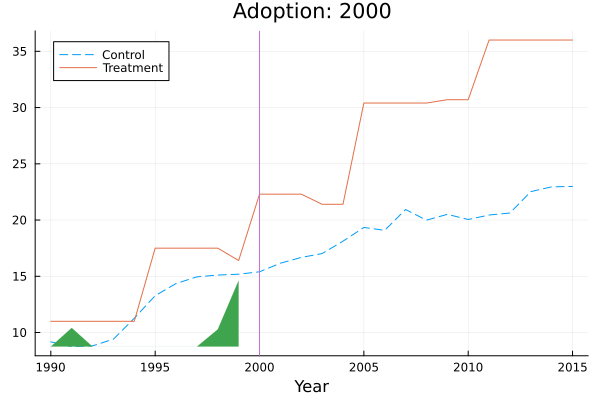
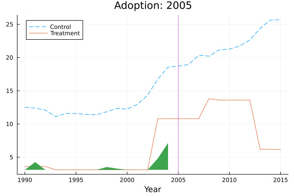
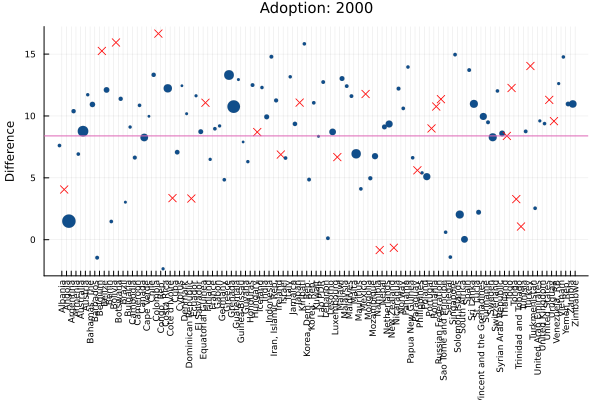
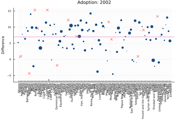
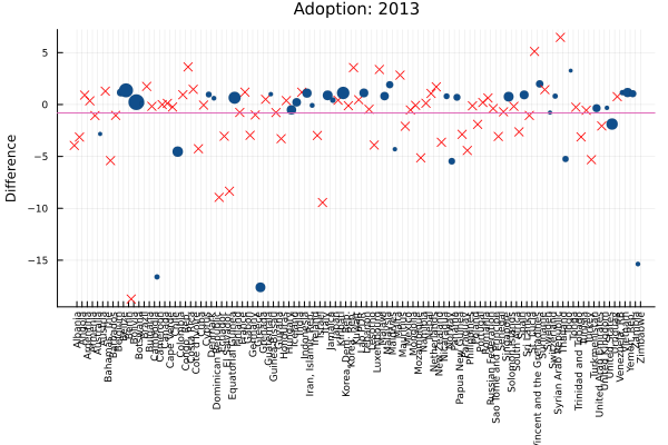
The dictionary design is specially useful for staggered treatment cases:

plots = plot_outcomes(data, :womparl, :country, :year, :quota)
plots["2000"]

plots["2002"]

plots["2003"]

plots["2005"]

plots["2010"]

plots["2012"]

plots["2013"]

plots = plot_weights(data, :womparl, :country, :year, :quota)
plots["2000"]

plots["2002"]

plots["2003"]

plots["2005"]

plots["2010"]

plots["2012"]

plots["2013"]

Dmitry Arkhangelsky, Susan Athey, David A. Hirshberg, Guido W. Imbens, and Stefan Wager. Synthetic Difference in Differences, American Economic Review, December 2021.

Damian Clarke, Daniel Pailañir, Susan Athey, and Guido Imbens. Synthetic Difference-in-Differences Estimation. Institute of Labor Economics Discussion Paper Series, January 2023.

Sebastian Kranz. Synthetic Difference-in-Differences with Time-Varying Covariates. January 2022.