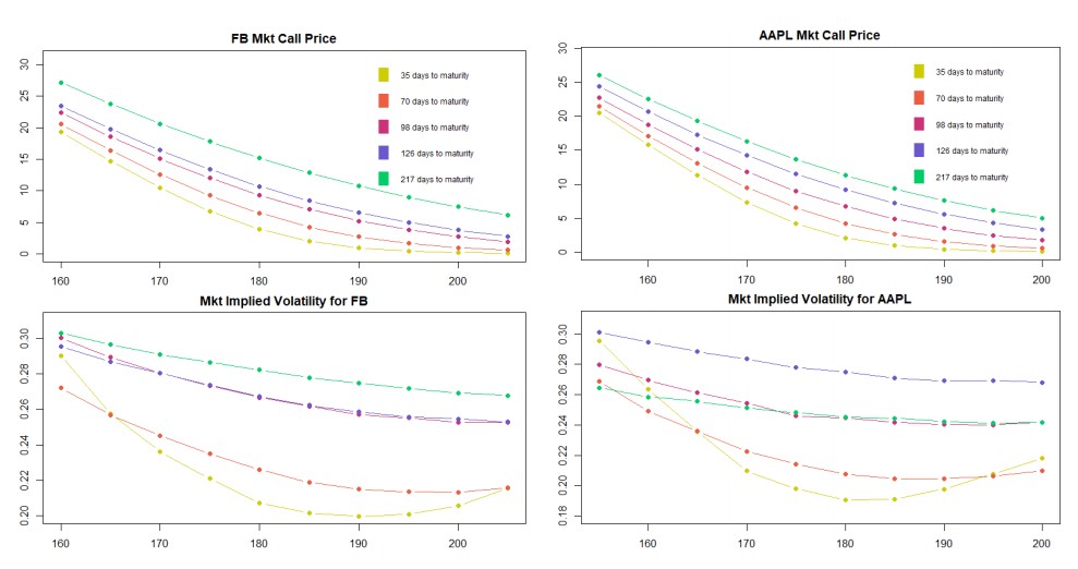
The types of equity are similar: both are stocks of related industries representing well established companies and show similar stock behavior. Their historical data provides us with a correlation of 0.451742. From asset derivative prices in the market we extract the implied volatilities and observe that smiles show different volatilities for different maturities, the smile, skew and smirk characteristics being the most defined for shortest time to maturity options as visualized in the graph below. For this evaluation and the succeeding model the environment is considered to be risk-free, with a risk-free rate set at rf = 0.01.

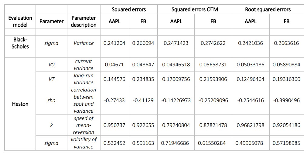
Calibration is performed for 2 models: Black-Scholes and Heston. For the first model we have to evaluate an appropriate volatility measure sigma σ. For Heston – 5 model defining parameters as used in the function callHestoncf (appendix 1b) from R package NMOF (based on the book "Numerical Methods and Optimization in Finance" by M. 'Gilli', D. 'Maringer' and E. Schumann, 2011): current variance v0, long-run variance vT, correlation between spot and variance rho, speed of mean-reversion k, volatility of variance sigma (value smaller than 0.01 is replaced with 0.01 by the modeled function). For calibration we are summing the squared errors between model and market prices and minimizing the result for both instruments and two models. For minimizing the sum of squared errors a modest-memory optimizer with bounds function in R package NMOF is used. Method "L-BFGS-B" is that of Byrd et. al. (1995) which allows box constraints for each variable. This uses a limited-memory modification of the BFGS quasi-Newton method. There have been some disconcerting failures of this method observed, but it often performs very well. 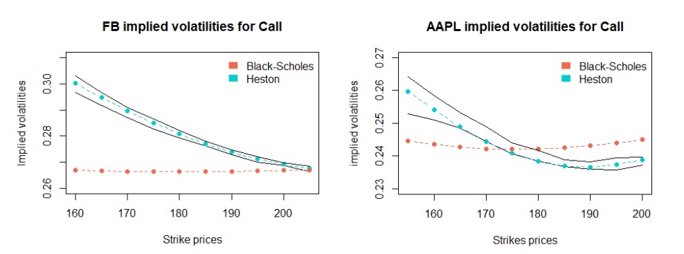The results shown for both models are calibrated using 5 maturities and 10 strike prices. For Black-Scholes the process presents us with one calibration measure – sigma. We see that this measure alone cannot mimic the market volatilities as well as Heston. Heston model gives us 5 parameters to vary since it accounts for stochastic volatility. Implied volatility surfaces for both models are shown below. From the graphs we can see that both models detour from the market implied volatility, but Black-Scholes has a more severe deviation, which is expected since the calibration is performed adjusting one parameter – sigma. Heston, on the other hand, does a much better work fitting between ask and bid spread due to the number of parameters it incorporates. Although it still does not catch all of the market movements. Root Squared Errors:

For all models, we consider the risk-neutral dynamics of the stock price, which might not represent the real world environment. Other assumptions are made, that will not be entirely correct in the market itself. We assume no seasonality, no behavioral bias. The Black-Scholes model is inconsistent with the observed smiles, skew and smirk of the implied volatility, it assumes constant volatility and normal Gaussian distribution of returns. Even though Heston model allows stochastic volatility movements, not all of the volatility movement features are represented in this model. The modeled function does not allow jumps (severe changes in the underlying asset price), clustering, differences between the severity of underlying asset value downfalls and rises. Going further to improve the model, we might also want to concentrate on out of the money options for valuation as incorporation of in the money value might construct a bias. Also another process than the geometric Brownian motion could be set to generate randomness. In addition, a more informed estimation and prediction of volatilities could be performed, since our results are based solely on the historical data. It would be naïve to assume that historical performance can directly predict the future values of the assets, which are influenced by the performance and technological progress of companies, political and macroeconomic influences. The Heston model is known to show its limitations for short dated options.  

For the Black-Scholes approach we use Monte Carlo simulation and perform Black-Scholes calculations for intermediate steps. For Heston, in order to price the path-dependent barrier options using the stochastic volatility models, Monte Carlo simulation is also performed. The process of the underlying is similar to the Brownian motion, but the volatility is stochastic: it follows a stochastic square root process. The two Brownian motions are also correlated. There is a risk that the variance process will take negative values due to the discretization of the processes. For that reason, in each time step, the function makes sure that parameter VT is non-negative. We compute the Delta, Gamma, Vega and survival probability of this option.

The delta (∆) is a measure of sensitivity of the changing option value with respect to the changing underlying stock price S. Deltas of knock-out options tend to differ from those of ordinary options. Generally, we observe that near the barrier, the graphs of the knock-out options have kinks. This is what complicates hedging of these options near the barrier. Equation is normally expressed as a percentage. Delta hedging aims to minimize Delta risk (make it equal to zero). From our models we see that the price of the option should change 0.01-0.02 USD. One can delta-hedge a long position of the option by selling ∆-shares of stock and investing the rest of the money in a risk-free financial institution such as a bank. Let’s assume that a seller uses Heston pricing and evaluates the option at 1.33 USD per share: if we buy 10 options for 100 shares and pay 13300 USD, we have to sell (or go short on) stock worth ∆ * 13300 = 1268,15 USD. * 177 = 224462.55 Pricing and Hedging of Barrier Options

A more sophisticated hedge would be Static hedging: it involves the construction of a portfolio that contains the underlying call option and other options (calls and/or puts) with different expiry dates, same strikes and with fixed weights. It is possible to construct such a portfolio such that it replicates the value of the target option for any underlying stock price for a wide period of time before maturity, without any need for rebalancing (changing the weights). The value of this hedging portfolio ought to be the same as that of the target option at the barrier and maturity. Unlike delta-hedging, the risk and costs are minimized in the sense that the investor does not have to trade during the option’s life span. This construction would require sophisticated calculations, but may well be a better option, especially since Deltas of a barrier option tend to have kinks that are not common for vanilla options and might be hard to replicate and track.

The valuation process of parameters for the models in itself has flaws discussed above. All the risks from estimation are still valid. In addition, we find that repeating the regressions, the model results vary, therefore it would be beneficial to increase the number of simulations and steps. Furthermore, human error starts to become more and more dangerous as well as possible.

You have to price an exotic option that pays at maturity T , the maximum between AAPL (S1(T )) and FB (S2(T )) (minus a strike price K). Precisely, the payoff is defined by: (max(S1(T ); S2(T )) - K)+ where S1(0) = 175 USD is the value of AAPL at 2 pm, S2(0) = 178 USD is the value of FB at 2 pm. We use Monte Carlo simulation with Black-Scholes option valuation for 10000 simulations and 500 steps. 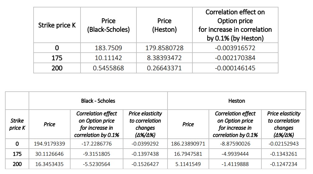The results are displayed in the table below for three strikes and 2 pricing models. The correlation effect is a marginal measure that calculates the relationship between a difference in price of two models (one with increased correlation between underlying assets by 0.1%) and the difference in correlation. The correlation effect is inverse, which means that the by increasing option correlation we are decreasing the price of option. This is expected due to the fact that as the underlying assets converge to same behavior, the options become less risky and therefore less expensive.

We observe that the option prices are reasonable and can be assumed that the models can both be implemented in valuation process. Nevertheless, some additional measures could be incorporated in the models as mentioned above in the previous descriptions. All the weaknesses that were discussed above also apply. Correlation, model estimations and predictions depend on technicalities, assumptions, which can be hard to forecast or evaluate. And there will always be a risk to not predict the future.