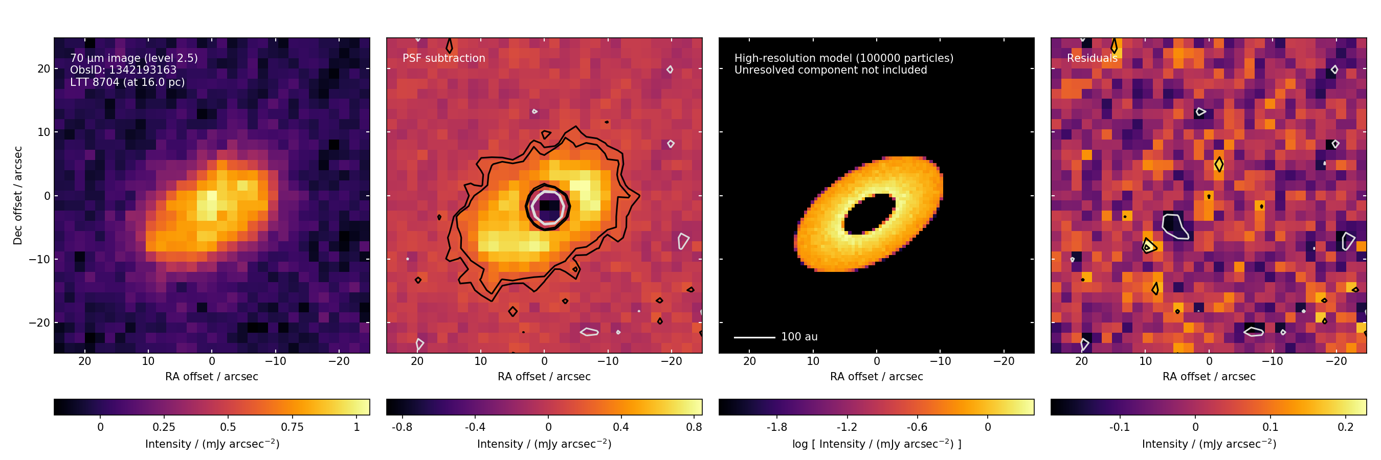
Fit a debris disc model to a Herschel PACS image. The code here is an extension of that used to model the disc of HD 95698 in this paper: 2019MNRAS.488.3588Y.

Fitting is performed by the script pacs_model.py. You can either import the file and call the run function, or run the script from the command line and pass arguments that way. The only required argument is name_image, which should be a string pointing towards the FITS file containing the data that need fitting. The optional arguments allow you to control the details of the fit (e.g. model resolution, number of iterations), and to provide extra information about the system of interest that will make the results more informative (e.g. distance, expected stellar flux). For full details of the optional arguments, run python pacs_model.py -h.

Optionally, an image to use as a PSF may be supplied. By default, an image of the calibration star γ Dra is used. This repository includes four such images, downloaded from the Herschel Science Archive, and the code will choose the appropriate one based on the processing level (2 or 2.5) and wavelength (70 or 100 μm) of the image to be analysed.

For fitting a large number of images, pacs_model_batch.py should be helpful. This script reads in a CSV file (obs_path_list.csv) containing information about the images to fit and calls run for each system. An appropriately formatted CSV can be produced with the help of the notebook get_obs_paths.ipynb. However, pacs_model_batch.py could be easily modified to read in a CSV with less information and make use of the default argument values.

Finally, gather_images.py can be used to sort the output of pacs_model_batch.py into folders containing systems that the code classified as unresolved, succeeded and failed. The classification is based on an Anderson-Darling test, which determines whether the PSF-subtracted image and model residuals are consistent with Gaussian noise. Browsing the images in these folders can be a good way to get an overview of the fitting results for a large batch of systems.

For each system modelled, pacs_model.py will save:

• chains.pdf, chains.png: a plot showing the evolution of the MCMC walkers over time;
• corner.pdf, corner.png: a plot showing the 2D projections of the posterior model parameter distributions;
• image_model.png: a plot showing the image, PSF-subtracted image, best-fitting model and residuals;
• samples.pickle: a pickle containing the MCMC samples (excluding burn-in) for future analysis;
• params.pickle: a pickle containing the key results of the fit.

You can find some example output for HD 207129 / LTT 8704 and AU Mic in this repository.

If run receives test = True, the code will first try to check whether the image is consistent with a point source, and skip the disc fit if so (see the function Plottable.consistent_gaussian for details). In this case, image_model.png will only contain the first two panels, and the MCMC-related output won't be produced.

There are two different methods available for generating disc models; which is used depends on whether run receives model_type = ModelType.Particle or model_type = ModelType.Geometric. In the first method, a number of particles are generated in the disc, and their positions are binned in the sky plane to obtain a synthetic image. The second method is purely geometric: the sky is divided up into pixels, and the physical distance from the star to the disc element at each pixel is calculated given the disc's proposed inclination and position angle.

The second model (but not the first) breaks down for edge-on discs, and hence the disc's inclination needs to be restricted to below 90 degrees if it is used. Restricting inclination to e.g. 88 degrees still allows AU Mic, a known edge-on disc, to be well modelled, but the breakdown close to 90 degrees does leave an imprint on the posterior inclination distribution (which can be seen by comparing the distributions produced using both models). Thus, in general I recommend using the first model, though if you are trying to fit a very large disc (in angular size) you will likely need to use a large number of particles npart (which comes with a performance hit) to limit the effect of shot noise.

The code models discs as having a single power-law radial surface brightness profile between an inner and outer radius. This is often a good approximation, but high signal-to-noise images of discs with more complicated radial profiles or asymmetries may require a more detailed model.

Disc parameters are sampled using the MCMC technique (via the emcee package).

Some features that it would be beneficial to add in the future:

• An option to include more than one point source in the model, to account for any nearby companions or background objects. Since the code currently doesn't do this, what generally happens in multiple-source images is that the best-fitting model has a disc whose ansae pass through at least one of the sources. These 'discs' can sometimes fit the data well, but are unlikely to be the true explanation of what's going on!

The code here (other than rebin.py, which is taken from the SciPy Cookbook) was written by Ben Yelverton. Please let me know if you find any issues. If you've found it helpful for any work you're planning to publish, I'd appreciate an acknowledgement. I am grateful to Grant Kennedy for advice on this work.