• Python
• Pandas
• GeoPandas
• Matplot
• Folium
• Git
• Markdown
• JSON
• NumPy
• .gitignore
• requirements.txt

1. USA Real Estate Data
2. Global Cost of Living
3. World Happiness Report 2021
4. World Happiness Ranking

This repo includes data manipulation for datasets working with a team. Alejandro performed profiling, cleaning and transformations on the Global Cost of Living, and exported to a clean version of the csv named cost_living.csv. Drew worked on profiling, cleaning and transformations for the World Happiness Report 2021 and World Happiness Ranking data sets to merge into world_happiness_clean.csv. Ruben performed profiling, cleaning and transformations on the USA Real Estate Data to compile clean_realtor_data.csv, and then joined the other contributors' datasets into one consolidated csv file. The realtor and cost of living data were concatenated in order to expand the data set for price per square meter data at the city level. Then that expanded data (cost_living_with_realtor.csv) set was merged with world_happiness_clean.csv into the consolidated cl_real_happiness.csv.

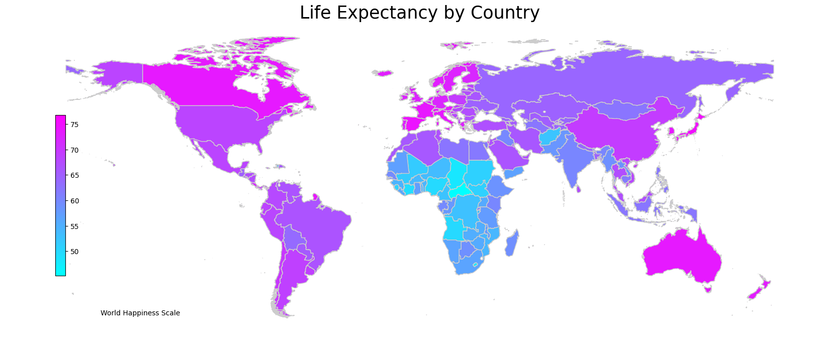
Once the datasets were cleaned and consolidated, the team created (and in some cases recreated) data visualizations and analysis using cl_real_happiness.csv. In the rg_maps.ipynb notebook is a geo heat map of life expectancy by country that was put together by Ruben. Below is the output of the visualization:

Drew put together a pie chart highlighting the life expectancy for the top 10 countries. Code for the visualization is located in dw.ipynb. Below is the pie chart:

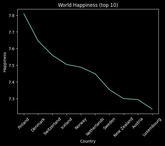
Drew also put together a line graph highlighting the happiness score for the top 10 countries. Interesting note is there seems to be correlation between Happiness and Life Expectancy with the two showing the same exact top ten countries. Code for the visualization is located in dw.ipynb. Below is the line chart:

Drew compiled a map highlighting the happiness score for all countries. Code for the visualization is located in dw.ipynb. Below is the output of the visualization:

Alejandro put together a map visualization using Folium, that shows the average price per square meter by state. Code for the visualization is located in alex_work.ipynb. Below is a snapshot of the visualization, as it is a dynamic map so in the notebook you can zoom in and out:

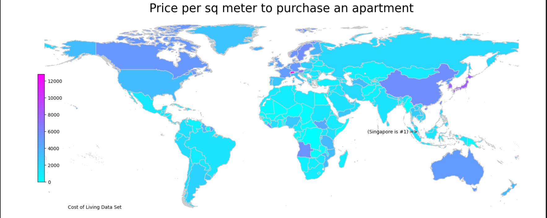
Alejandro also used geopandas to create a similar map on a global scale:

Ruben created a scatter plot visualization that shows the average price per square meter against life expectancy and social support, for 10 countries with the highest life expectancy. Code for the visualization is located in rg_scatter.ipynb. Below is a snapshot of the visualization:

Overall, the team was able to limit the amount of merge conflicts by working on independent notebooks and assigning different tasks (e.g. Each focused on different data sets, Ruben completed README, etc.). One challenge that we underwent was version control for the datasets that were transformed and then needed to be leveraged by the broader group. One key learning we had was going forward a good practice to help mitigate this is to spend time as a group validating the final data set, agree its ready to be leveraged, and then go on to begin our data visualizations and exploration. This would prevent having version control issues and digging through code to ensure its reading from proper csv files.

• Go to https://github.com/apsocarras/team-week.git to find the specific repository for this website.
• Then open your terminal. I recommend going to your Desktop directory:

  cd Desktop

• Then clone the repository by inputting:

  git clone https://github.com/apsocarras/team-week.git

• Go to the new directory or open the directory folder on your desktop:

  cd python-team-week

• Once in the directory you will need to set up a virtual environment in your terminal:

  python3.7 -m venv venv

• Then activate the environment:

  source venv/bin/activate

• Install the necessary items with requirements.txt:

    pip install -r requirements.txt

• Download the necessary csv files listed in the Datasets Used section
• Download the cleaned up csv files created by the contributors on this google drive
• One all csv data sets have been added to the data folder in this directory, you can open it
• With your virtual environment now enabled with proper requirements, open the directory:

  code .

• No known bugs

MIT License

Copyright (c) 2022 Ruben Giosa, Alejandro Socarras, Drew White

Permission is hereby granted, free of charge, to any person obtaining a copy of this software and associated documentation files (the "Software"), to deal in the Software without restriction, including without limitation the rights to use, copy, modify, merge, publish, distribute, sublicense, and/or sell copies of the Software, and to permit persons to whom the Software is furnished to do so, subject to the following conditions:

The above copyright notice and this permission notice shall be included in all copies or substantial portions of the Software.

THE SOFTWARE IS PROVIDED "AS IS", WITHOUT WARRANTY OF ANY KIND, EXPRESS OR IMPLIED, INCLUDING BUT NOT LIMITED TO THE WARRANTIES OF MERCHANTABILITY, FITNESS FOR A PARTICULAR PURPOSE AND NONINFRINGEMENT. IN NO EVENT SHALL THE AUTHORS OR COPYRIGHT HOLDERS BE LIABLE FOR ANY CLAIM, DAMAGES OR OTHER LIABILITY, WHETHER IN AN ACTION OF CONTRACT, TORT OR OTHERWISE, ARISING FROM, OUT OF OR IN CONNECTION WITH THE SOFTWARE OR THE USE OR OTHER DEALINGS IN THE SOFTWARE.