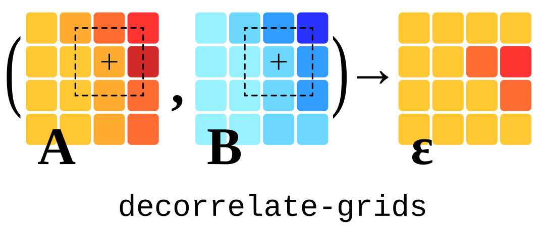
Provided with two 2-D labelled arrays ( $\mathbf{A}, \mathbf{B}$ "grids"), perform a windowed linear regression between the two and return the fitted coefficients, as grids. The aim is pursuing the removal of any (linearly) correlated component between the data in $\mathbf{A}$ and $\mathbf{B}$, assuming that their linear relationship varies spatially - hence the rolling window. Array $\mathbf{\epsilon}$ is an array of "regression residuals", the result of subtracting the fitted relationship from $\mathbf{A}$.

This was designed with a specific application in mind: mitigation of tropospheric delays in Interferometric Synthetic Aperture Radar (InSAR) data (see e.g. Bevis et al., 1992; Tymofyeyeva and Fialko, 2015; Adam, 2019; and chapter 4.6 in ESA EGMS Algorithm Theoretical Basis Document, 2021). There, the unwrapped phase (the response variable, in the context of regression) is observed to be correlated with topography (an explanatory variable), a phenomenon which can be attributed in part to non-modelled propagation delays. Among the mitigation strategies, the unwrapped phase can be de-correlated with respect to topography. Ideally, with all the due simplification of this context, this would reveal only the phase caused by deformation of the Earth surface. This was actually set up to test if this is effective and how does it compare to other strategies.

However, no part of this package is InSAR-specific. The procedure can be applied to any data with similar goals of de-correlation. Using the result of windowed regression by itself is also a possibility, as it is customarily done in some applications (e.g. topography-gravity regression in geophysics, see e.g. Pivetta and Braitenberg, 2020). Nevertheless, some assumptions and implementation choices reflect our original aim. Chiefly, data formats: the script reads and writes netCDF files, using xarray. The core procedure works regardless of this, hence moving on to a format-agnostic implementation is in the To Do list.

At the moment, only ordinary-least-squares linear regression is implemented as "correlation model". We deemed this enough for the application we were concerned with. Extension to other models or refactoring to allow any function to be used would be an interesting improvement.

Assuming variable $a$ and $b$ are in a relation in the form:

$$a(b) = f(b) + \epsilon$$

our goal is to estimate $f(b)$, thus the regression residuals $\epsilon$.

We choose a simple linear model for $f(b)$:

$$f(b) = c_0 + b * c_1$$

and we will assume that in each neighbourhood of an element in our arrays this is the model describing the unwanted "correlated component" of the observed signal $a$.

The least square system for each $\mathbf{A}(i, j)$, $\mathbf{B}(i, j)$ element of the input arrays, which share the same $m \times n$ size, is:

$$\hat{A}_{i, j}^{o, p} = c_{0_{i, j}} + \hat{B}_{i, j}^{o, p} * c_{1_{i, j}}$$

where $\hat{A}_{i, j}^{o, p}$ and $\hat{B}_{i, j}^{o, p}$ are each a vector of $\mathbf{A}$ and $\mathbf{B}$ elements in the neighbourhood (rolling window) of $i, j$, defined by a "window half width" of $m, n$ rows and columns:

$$ \hat{A}_{i, j}^{o, p} = \left[ a_{i-o, j-p}, \dots, a_{i+o, j-p}, \dots, a_{i-o, j+p}, \dots, a_{i+o, j+p} \right] $$

Note that we are using a boxcar-shaped window, but the weights of any windowing function may be employed in a weighted least squares scheme.

No regression is carried out on elements on the edges (where one or more of the following is true: $i-o < 0$, $i+o > m$, $j-p < 0$, $j+p > n$) and elements in which $\mathbf{A}(i, j)$ or $\mathbf{B}(i, j)$ is $\mathtt{NaN}$.

We used $c$ for denoting the regression parameters, rather than the commonly used $\beta$, for familiarity with $c$ as in coefficients.

This left with a risk of confusion with the residuals matrix, which could not be $\mathbf{C}$ - since we do have arrays of fitted coefficients. Notation clashes arose for any other letter we thought of (e.g. $\mathbf{R}$, but there is an array of $r$ coefficients of determination). Since $\epsilon$ is used in some places for regression residuals, we went with that (e.g. $Y = X \beta + \epsilon$ in Hastie et. al, Elements of statistical learning, Eq. 3.23).

Arguably, the logo graphics would have been nicer as $(\mathbf{A}, \mathbf{B}) \rightarrow \mathbf{C}$.

At this stage, this boils down to:

1. Clone this repository:

git clone https://github.com/apasto/decorrelate-grids.git && cd decorrelate-grids

2. Install the package, e.g. with pip or by creating an ad hoc Conda environment:

• pip: pip install -e ./
• conda: conda env create -f environment.yml, then activate it

3. To print out a short usage help of the provided decorrelategrids cli tool:

decorrelategrids -h

This is currently at a working, but early stage. Some steps are planned to get beyond the prototype state, see this task list: issue #2.

This work is licensed under the Apache License 2.0. See LICENSE.