This (small) package is a finite volume solver for the Self-Organized Hydrodynamics (SOH) partial differential equation system derived as the macroscopic limit of a Vicsek-like model by P. Degond and S. Motsch in
[1] P. Degond, S. Motsch. Continuum limit of self-driven particles with orientation interaction, Math. Models Methods Appl. Sci., Vol. 18, Suppl., pp. 1193-1215, (2008).
The implementation is based on the methodology developed by S. Motsch and L. Navoret in
[2] S. Motsch, L. Navoret, Numerical simulations of a non-conservative hyperbolic system with geometric constraints describing swarming behavior, Multiscale Model. Simul., Vol. 9, No. 3, pp. 1253–1275, (2011).
The Fortran package Vicsek_macro is an earlier version of this solver implemented by S. Motsch.
This package can be installed globally using the Julia package manager by typing
] add https://github.com/antoinediez/SOH.jl.gitAlternatively, it is also possible to clone the GitHub repository and to run a simulation as explained in the example script example.jl.
The SOH model is a continuum version of the interacting particle system, originally introduced by Vicsek et al. in
[3] T. Vicsek, A. Czirók, E. Ben-Jacob, I. Cohen, O. Shochet, Novel type of phase transition in a system of self-driven particles. Phys. Rev. Letr., Vol. 7, No. 6, pp. 1226, (1995),
and further developed in [1]. This swarming model is based on an alignment mechanism which tends to relax the direction of motion of each particle towards the average direction of motion of its neighbours. The particles are assumed to be self-propelled and to move at a constant speed, which is a specificity of the Vicsek model.
The SOH system reads
ρ(∂ₜΩ + c₂(Ω⋅∇ₓ)Ω) + λP(Ω)(∇ₓρ + ρ∇ₓV) = 0,
where ρ≡ρ(t,x) represents the density of particles and Ω≡Ω(t,x) is the velocity field at time t and at a position x∈R². The constant speed constraint is preserved thanks to the operator P(Ω) = Id - Ω⊗Ω which is the projection operator on the orthogonal of the vector Ω. It ensures that, for all (t,x),
provided that it holds at initial time.
The coefficients c₁, c₂ and λ are generic nonnegative constants. In [1,2], they are obtained as functions of a concentration parameter κ which defines the strength of the alignment between the particles. Different functions can be obtained with a different alignment mechanism, see for instance the one introduced in
[4] G. Dimarco, S. Motsch, Self-alignment driven by jump processes: Macroscopic limit and numerical investigation, Math. Models Methods Appl. Sci., Vol. 26, No. 7, pp. 1385–1410, (2016).
In all cases, the coefficients typically satisfy c₁>c₂ and λ = 1/κ.
The implementation is based on the methodology introduced by [2]. When V=0, the SOH model is shown to be the formal relaxation limit ɛ → 0 of a conservative system:
ɛ(∂ₜ(ρΩ) + c₂∇ₓ⋅(ρΩ⊗Ω) + λ∇ₓρ) = ρ(1-|Ω|²)Ω,
Following this idea, the finite volume scheme is based on a splitting method described by the following steps.
- Solve the conservative part
∂ₜ(ρΩ) + c₂∇_x⋅(ρΩ⊗Ω) + λ∇ₓρ = 0,
which is a classical 2D Euler system (with coefficients c₁≠c₂). Using a dimensional splitting method as described in Section 19.5 of
[5] R. J. LeVeque, Finite volume methods for hyperbolic problems, Cambridge university press, 2004, ISBN 0-511-04219-1,
this reduces to solving two 1D Euler systems. For this system, the present package implements a classical Roe scheme (as in the package Vicsek_macro) as well as a more stable positivity preserving HLLE scheme described in [5, Section 15.3.7] and introduced in
[6] B. Einfeldt, C. D. Munz, P. L. Roe, B. Sjögreen, On Godunov-type methods near low densities, J. Comput. Phys., Vol. 92, No.2, pp. 273-295, (1991).
- The relaxation part reads
ɛ∂ₜ(ρΩ) = ρ(1-|Ω|²)Ω,
It can be solved explicitly |Ω|² = 1/(1+C₀exp(-2/ɛt)) with C₀ = (1/|Ω₀|²-1). Numerically, taking the limit ɛ → 0 yields to a mere normalization
- Using again a fractional splitting [5, Section 17.1], the source terms reads
∂ₜΩ = λP(Ω)F, F=-∇ₓV
This part can also be solved explitly in dimension 2, namely Ω(t) = (cos(θ),sin(θ))ᵀ where
where F = |F|(cos(ψ),sin(ψ))ᵀ and C₀ = tan((θ₀-ψ)/2).
Finally, at each step, the boundary conditions are treated using the ghost-cell method described in [5, Chapter 7]. The boundary conditions currently implemented are either periodic, Neumann or reflecting boundary conditions.
The typical workflow to run a simulation is described in the example script example.jl which can be launched by typing
include("example.jl")This script defines some simulation parameters and runs the main function run! (defined in the script run.jl). In addition to running the simulation, this function also creates a new directory in the current path and save the data, heatmap plots and a video. All the plots and videos are produced using the Makie.jl package. The data are saved using the JLD2 package.
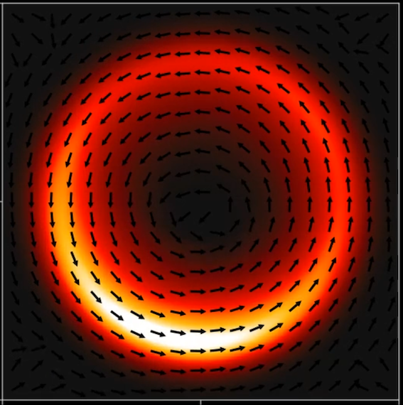
In the example script, the density is initially uniform and the velocities are uniformly randomly sampled. The system is subject to reflecting boundary conditions and to a confining radial potential in a disk, namely the potential is given by V(r) = 0 for r<r₀ and V(r) = (C/2)(r-r₀)² for r>r₀. It leads to a final milling state as shown in the following video.
mill_SOH.mp4
For analytical results in this direction, see for instance
[7] P. Degond, H. Yu, Self-organized hydrodynamics in an annular domain: Modal analysis and nonlinear effects, Math. Models Methods Appl. Sci., Vol. 25, No. 3, pp. 495–519, (2015).
On a grid of size 400x400, one iteration takes less than 0.1 seconds of CPU time on an Intel MacBook Pro (2GHz Intel Core i5 processor with 8GB of memory). With this configuration, it takes about 15 minutes to run the example script. It is slighlty more performant (about 50% faster) than the Fortran implementation. The simulation time is comparable to the one needed to simulate of a system of 100k particules on a CPU or of several millions of particles on a GPU, both using the high-performance SiSyPHE library.
Note: currently, a significant computational time is necessary to save plots or to produce a video. The simulation is about two times faster when no plots are generated.
