The Notre Dame Fighting Irish will beat the Louisville Cardinals on September 2, 2019, but the Fighting Irish should not take this game lightly. Of the 1,000,000 games they have played over a 10 minute period, the Irish have won only 623,499 of those games.

Let's dive into how simulation and other techniques are coordinated to generate this prediction. We R going to be using the R programming language.

This analysis requires 3 packages:

• Tidyverse - Awesome data bending/mashing tools
• rvest - Web Scraping
• fitdistrplus - As my neighbor Cheapskate Charlie says, "I ain't payin' no $2,530 for some excel add-on!"

Before we simulate these games, we need data on historical performance. Scores were scraped from some website. The data is downloadable here (for Brian Kelly) and here (for Scott Satterfield). For semi-transparency, below are two functions used to gather and clean our data.

GetGameScores <- function(INPUT_YEAR, INPUT_TEAM){
  templist <- list() 
  for(year in INPUT_YEAR){    
    url <- paste0("HTTPS:https://WWW.HOMEPAGE_HERE/", INPUT_TEAM ,
                  "/MORE_WORDS_HERE/", year ,"/URL.COM")
    temp <- url %>%
      read_html() %>%
      html_nodes(xpath='xpath to the data table goes here') %>%
      html_table() %>%
      as.data.frame()
    templist[[year]] <- temp
  }
  OUTPUT.GetGameScores <- bind_rows(templist)
  return(OUTPUT.GetGameScores)
}

GetGameScores() will scrape game results for a specified team across a specified date range.

CleanGameScores <- function(INPUT, CapacityLimit){
    mutate(GameMonth = case_when(substr(Date,1,2) == "08" ~ "August",
               					 substr(Date,1,2) == "09" ~ "September",
               				     TRUE ~ as.character(Date))
          ) %>%
    separate(Result,c("PtsFor","PtsAgainst"), sep = "-") %>%
    mutate(PtsForAdj = ifelse(Attendance >= CapacityLimit , PtsFor , PtsFor * 0.70),
           PtsAgainstAdj = ifelse(Attendance >= CapacityLimit , PtsAgainst , PtsAgainst * 0.70))
}

CleanGameScores() will reformat the data and create our Adjusted Points. In my execution, I set my CapacityLimit argument to 40,000. Any game played in the presence of 40,000 attendees or less will have its points multiplied by 70%.

Years.BK <- as.character(c(2010:2018)) #Brian Kelly Coaching Years at ND
Years.SS <- as.character(c(2013:2018)) #Scott Satterfield Total Coaching Years

temp.BrianKellyRawScores <- GetGameScores(Years.BK, "Notre Dame")
Scores.BrianKelly <- CleanGameScores(temp.BrianKellyRawScores)

temp.ScottSattRawScores <- GetGameScores(Years.SS, "Notre Dame")
Scores.ScottSatt <- CleanGameScores(temp.ScottSattRawScores)

All 9 years of Brian Kelly's games at Notre Dame was scraped. Scott Satterfield will enter his first year as head coach of Louisville, but he has 6 years of total head coaching experience.

Scott Satterfield was the QB coach and offensive coordinator of the 2007 Appalachian State team. I was eating a jalapeno and turkey sandwich with my roommate while watching Appalachian State pummel Michigan.

This section steps through our method of generating a predicted conclusion of Notre Dame's upcoming 2019 season opener. Topics covered include: distribution fitting, sampling, and winning.

To simulate our points, we fit these scores to a distribution, then sample from that distribution over many iterations. We could just randomly sample from existing scores, but that would be too easy. Let's crank it to 11. Let's strive to inspire.

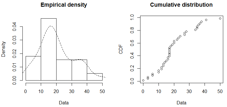
Since we're simulating a season opener, I will subset our data to only games played in August and September. Initial eye-ball test showed a positive-ish skew to Brian Kelly's August/September points gained and his points against.

plotdist(BK.AugSept$PtsForAdj , histo = TRUE , demp = TRUE)    
plotdist(BK.AugSept$PtsAgainstAdj , histo = TRUE , demp = TRUE)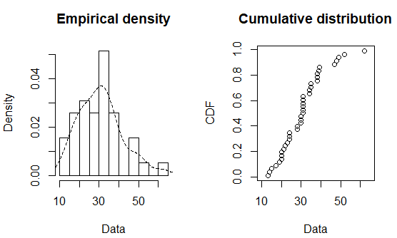 

After trying a few distribution comparisons, our CDF plot shows that the distribution of Coach Kelly's "Points For" scores most closely fit either a lognormal or gamma distribution. AIC was used as the deciding factor -- the gamma fit has the lowest AIC.

fitND.ln <- fitdist(BK.Scores$PtsForAdj , "lnorm")
fitND.g <- fitdist(BK.Scores$PtsForAdj , "gamma")

denscomp(list(fitND.w, fitND.ln, fitND.g))
cdfcomp(list(fitND.w, fitND.ln,fitND.g)) 

summary(fitND.ln)
summary(fitND.g)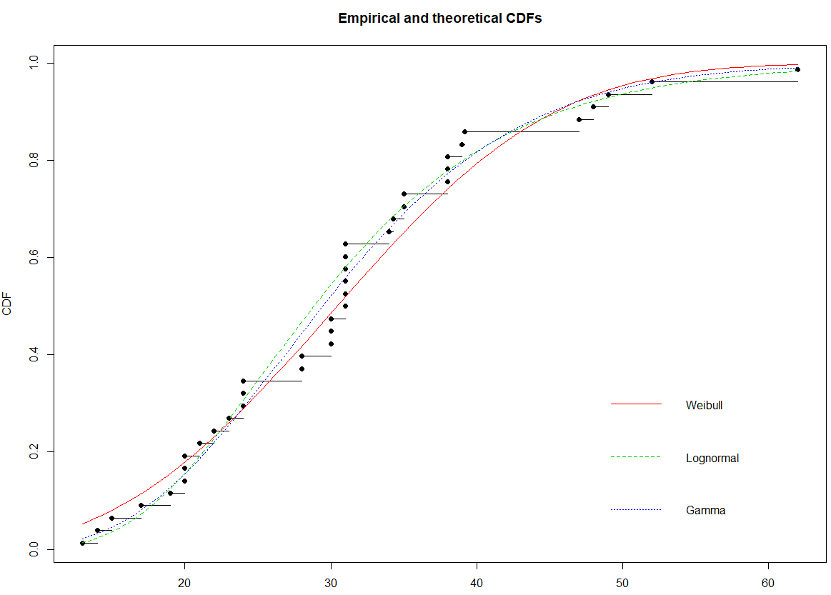

This process is repeated 3 more times for the following events:

• Brian Kelly's "Points Against" data
• Scott Satterfield's "Points For" data
• Scott Satterfield's "Points Against" data

With respect to the distribution fitting shown above, the rgamma() function in base-R will randomly sample from a gamma distribution. This function will be used to generate our simulated scores. Be sure to complete the shape and rate arguments, as determined from the distribution fitting. Note: My 1,000,000 iterations may be excessive, but it allows for an attention grabbing header.

fitND.g <- fitdist(BK.Scores$PtsForAdj , "gamma")

rand.ND_PF <- rgamma(n = 1000000,
                     shape = fitND.g$estimate[[1]],
                     rate = fitND.g$estimate[[2]]
                     )

Repeat this process 3 more times for the 3 remaining distributions.

The distribution-specific sampling outputs must be assembled to provide a complete prediction.

Game scores for both teams are determined by combining the simulated Points For and Points Against. As an example: the Notre Dame score is determined by combining the simulated Notre Dame Points For with the Louisville Points Against. This execution applies an 80/20 weighting, biased toward Points For. After developing the Notre Dame score and the Louisville score, a simple boolean statement comparing ND vs Louisville can be written to determine a ND victory.

sim.tempbind <- cbind(sim.ND_Scores , sim.L_Scores) %>%
  apply(2 , function(x) ifelse(x < 0 , 0 , x)) %>%
  as.data.frame() %>%

  mutate(ND_Score = (rand.ND_PF * 0.8) + (rand.L_PA * 0.2),
         Lou_Score = (rand.L_PF * 0.8) + (rand.ND_PA * 0.2),

         ND_Victory = ifelse(ND_Score > Lou_Score , 1 , 0))

#WIN OUTCOME: ND vs Louisville
table(sim.tempbind$ND_Victory)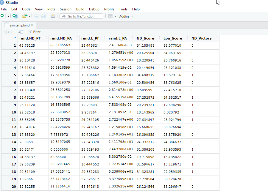

Inspecting the proportions of 1s (ND victory) and 0s (ND loss) in the column ND_Victory will produce our final result. In this execution, Notre Dame won 62.3% of the simulated games.

> #WIN OUTCOME: ND vs Louisville
> prop.table(table(sim.tempbind$ND_Victory))

       0        1 
0.376501 0.623499 

Game attendance was used as a fuzzy proxy for strength of schedule, but it does not account for situations where a Power 5 team defeats a smaller school at home. For example: Notre Dame's 2018 home victory against Ball State should not be weighted the same as their 2017 home blow-out against USC, despite both being played in the presence of 80,000 fans. An improvement would be to have the simulation also handle home game victories against non-Power 5 opponents.