![]()

WaterLily.jl is a simple and fast fluid simulator written in pure Julia. This is an experimental project to take advantage of the active scientific community in Julia to accelerate and enhance fluid simulations. Watch the JuliaCon2021 talk here:
WaterLily.jl solves the unsteady incompressible 2D or 3D Navier-Stokes equations on a Cartesian grid. The pressure Poisson equation is solved with a geometric multigrid method. Solid boundaries are modelled using the Boundary Data Immersion Method. The solver can run on serial CPU, multi-threaded CPU, or GPU backends.
The user can set the boundary conditions, the initial velocity field, the fluid viscosity (which determines the Reynolds number), and immerse solid obstacles using a signed distance function. These examples and others are found in the examples.
We define the size of the simulation domain as nxm cells. The circle has radius m/8 and is centered at (m/2,m/2). The flow boundary conditions are (U=1,0) and Reynolds number is Re=U*radius/ν where ν (Greek "nu" U+03BD, not Latin lowercase "v") is the kinematic viscosity of the fluid.
using WaterLily
function circle(n,m;Re=250,U=1)
    radius, center = m/8, m/2
    body = AutoBody((x,t)->√sum(abs2, x .- center) - radius)
    Simulation((n,m), (U,0), radius; ν=U*radius/Re, body)
end
The second to last line defines the circle geometry using a signed distance function. The AutoBody function uses automatic differentiation to infer the other geometric parameter automatically. Replace the circle's distance function with any other, and now you have the flow around something else... such as a donut or the Julia logo. Finally, the last line defines the Simulation by passing in parameters we've defined.
Now we can create a simulation (first line) and run it forward in time (third line)
circ = circle(3*2^6,2^7)
t_end = 10
sim_step!(circ,t_end)
Note we've set n,m to be multiples of powers of 2, which is important when using the (very fast) Multi-Grid solver. We can now access and plot whatever variables we like. For example, we could print the velocity at I::CartesianIndex using println(circ.flow.u[I]) or plot the whole pressure field using
using Plots
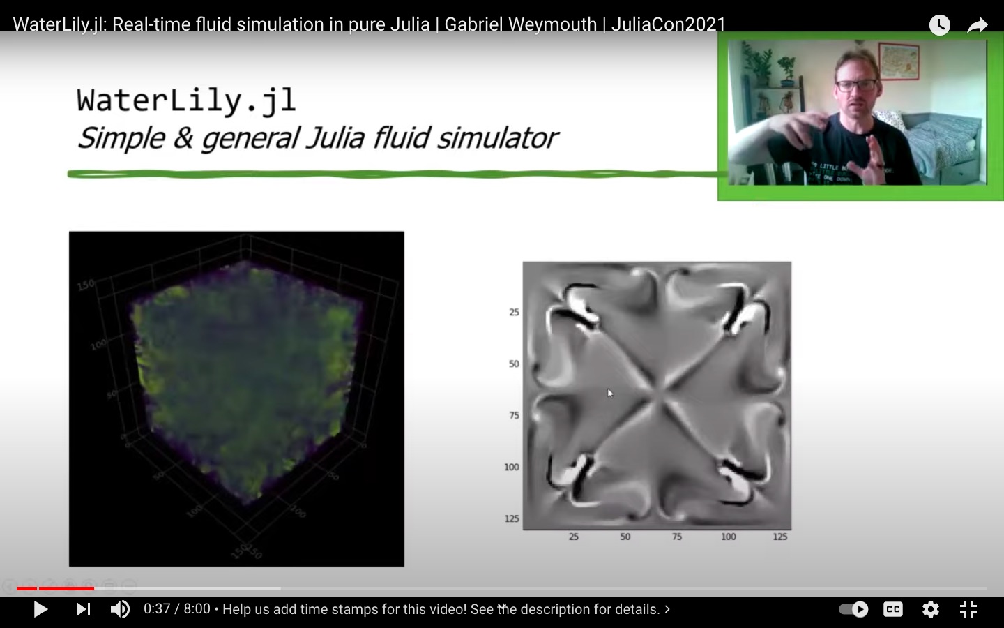
contour(circ.flow.p')A set of flow metric functions have been implemented and the examples use these to make gifs such as the one above.
The three-dimensional Taylor Green Vortex demonstrates many of the other available simulation options. First, you can simulate a nontrivial initial velocity field by passing in a vector function uλ(i,xyz) where i ∈ (1,2,3) indicates the velocity component uᵢ and xyz=[x,y,z] is the position vector.
function TGV(; pow=6, Re=1e5, T=Float64, mem=Array)
    # Define vortex size, velocity, viscosity
    L = 2^pow; U = 1; ν = U*L/Re
    # Taylor-Green-Vortex initial velocity field
    function uλ(i,xyz)
        x,y,z = @. (xyz-1.5)*π/L               # scaled coordinates
        i==1 && return -U*sin(x)*cos(y)*cos(z) # u_x
        i==2 && return  U*cos(x)*sin(y)*cos(z) # u_y
        return 0.                              # u_z
    end
    # Initialize simulation
    return Simulation((L, L, L), (0, 0, 0), L; U, uλ, ν, T, mem)
end
This example also demonstrates the floating point type (T=Float64) and array memory type (mem=Array) options. For example, to run on an NVIDIA GPU we only need to import the CUDA.jl library and initialize the Simulation memory on that device.
import CUDA
@assert CUDA.functional()
vortex = TGV(T=Float32,mem=CUDA.CuArray)
sim_step!(vortex,1)
For an AMD GPU, use import AMDGPU and mem=AMDGPU.ROCArray. Note that Julia 1.9 is required for AMD GPUs.

You can simulate moving bodies in Waterlily by passing a coordinate map to AutoBody in addition to the sdf.
using StaticArrays
function hover(L=2^5;Re=250,U=1,amp=π/4,ϵ=0.5,thk=2ϵ+√2)
    # Line segment SDF
    function sdf(x,t)
        y = x .- SA[0,clamp(x[2],-L/2,L/2)]
        √sum(abs2,y)-thk/2
    end
    # Oscillating motion and rotation
    function map(x,t)
        α = amp*cos(t*U/L); R = SA[cos(α) sin(α); -sin(α) cos(α)]
        R * (x - SA[3L-L*sin(t*U/L),4L])
    end
    Simulation((6L,6L),(0,0),L;U,ν=U*L/Re,body=AutoBody(sdf,map),ϵ)
end
In this example, the sdf function defines a line segment from -L/2 ≤ x[2] ≤ L/2 with a thickness thk. To make the line segment move, we define a coordinate tranformation function map(x,t). In this example, the coordinate x is shifted by (3L,4L) at time t=0, which moves the center of the segment to this point. However, the horizontal shift varies harmonically in time, sweeping the segment left and right during the simulation. The example also rotates the segment using the rotation matrix R = [cos(α) sin(α); -sin(α) cos(α)] where the angle α is also varied harmonically. The combined result is a thin flapping line, similar to a cross-section of a hovering insect wing.
One important thing to note here is the use of StaticArrays to define the sdf and map. This speeds up the simulation since it eliminates allocations at every grid cell and time step.
WaterLily uses KernelAbstractions.jl to multi-thread on CPU and run on GPU backends. The implementation method and speed-up are documented in our ParCFD abstract. In summary, a single macro WaterLily.@loop is used for nearly every loop in the code base, and this uses KernelAbstractactions to generate optimized code for each back-end. The speed-up is more pronounce for large simulations, and we've benchmarked up to 23x-speed up on a Intel Core i7-10750H x6 processor, and 182x speed-up NVIDIA GeForce GTX 1650 Ti GPU card.
Note that multi-threading requires starting Julia with the --threads argument, see the multi-threading section of the manual. If you are running Julia with multiple threads, KernelAbstractions will detect this and multi-thread the loops automatically. As in the Taylor-Green-Vortex examples above, running on a GPU requires initializing the Simulation memory on the GPU, and care needs to be taken to move the data back to the CPU for visualization. See jelly fish for another non-trivial example.
Finally, KernelAbstractions does incur some CPU allocations for every loop, but other than this sim_step! is completely non-allocating. This is one reason why the speed-up improves as the size of the simulation increases.
- Immerse obstacles defined by 3D meshes using GeometryBasics.
- Multi-CPU/GPU simulations.
- Add free-surface physics with Volume-of-Fluid or Level-Set.
- Add external potential-flow domain boundary conditions.
If you have other suggestions or want to help, please raise an issue on github.