Reproducible road safety research: an exploration of the shifting spatial and temporal distribution of car-pedestrian crashes
Dr Robin Lovelace — University of Leeds, Consumer Data Research Centre (CDRC) and Institute for Transport Studies (ITS) and Leeds Institute for Data Analytics (LIDA) 2019-02-01
This paper demonstrates a reproducible approach to download, format and analyse road crash data. Using the recently released stats19 R package, it is based on a dataset of half a million incidents (78,448 car-pedestrian crashes) from the UK STATS19 database, from 2013 to 2017. The analysis reveals variability in crash characteristics depending on social, environmental and regulatory factors, and variable police force performance in terms of ‘risk ratios’ over time. Geographic ‘small multiple’ visualisations show the potential of the approach to feed into interactive dashboards and maps to inform road safety policy, suggesting multiple directions for reproducible road safety research.
Keywords: geographic analysis, road safety, reproducibility
This paper is motivated by two high-level policy and academic objectives, which intersect. The policy objective is to provide high quality evidence and the ‘best available data’ in an ‘actionable’ form. The academic objective is to ensure that research findings can be reproduced, to ensure scientific falsifiability and encourage cooperation between researchers. These two objectives intersect because without reproducible methods it is difficult to generate high quality evidence that can be externally verified. Conversely, an academic environment that is conducive to collaboration and not competition requires a government that supports ‘open science’, “the transparent and accessible knowledge [and methods] shared and developed through collaborative networks” (Vicente-Saez and Martinez-Fuentes 2018).
This context is relevant to many fields of research that have practical and policy implications. Road safety research is no exception, as its findings often have direct policy implications and can be highly emotive, raising questions about the divide between research and policy (Elvik et al. 2009):
Can science and politics be kept apart in such a highly applied field of research? Where is the dividing line between science and politics in road safety?
More specifically, how can road safety research become more reproducible? This would clearly have advantages for many stakeholders: local and national governments would be better equipped to justify their road safety policies if the evidence on which they are based is the result of reproducible research conducive to ‘citizen science’ (Bonney et al. 2014); advocacy groups such as RoadPeace would be able to engage not only in lobbying, but also science, encouraging arguments from all sides to be based more on objective evidence, rather than emotive anecdote; and citizens themselves should benefit, from better road safety policies and the educational opportunities created by open science.
A more mundane motivation was that dozens of researchers are duplicating
effort by cleaning road crash data, a process first undertaken by one of
the authors three years ago (Lovelace, Roberts, and Kellar 2016) (the
code used to clean the data can still be found on
GitHub). The problem is that
the official source of road crash data, called STATS19 (Department for
Transport 2017), is provided in a series of opaque .csv files, which
provide only integer values. This has meant that, instead of pooling
data cleaning resources and focussing on the data analysis and research,
much time is spent doing data cleaning, duplicating previous work. To
solve this problem, the stats19 package was developed, which
automatically downloads and formats STATS19 data. Written in the popular
statistical programming language R (R Core Team 2019), stats19 was
published on the Comprehensive R Archive Network (CRAN) in January 2019
(Lovelace et al. 2019).
stats19 can convert the non-geographic data into a geographic representation of the crashes, an important feature given that much recent road safety research has been conducted using Geographic Information Systems (GIS) software (e.g. Kim and Levine 1996; Peled and Hakkert 1993; Steenberghen et al. 2004; Razzak, Khan, and Jalal 2011). With the growth of open source GIS products such as QGIS, this is a trend that can encourage open science, as defined above. A limitation of dedicated GIS software products from a reproducibility perspective, however, is that they tend to be based on a graphic user interface (GUI), rather than a command-line interface (CLI). This has led to many efforts to push geographic research in more reproducible and computational directions, under labels such as Geographic Information Science (GIScience), Geographic Data Science, and Geocomputation (Lovelace, Nowosad, and Meunchow 2019).
This paper ‘practices what it preaches’ in terms of reproducibility:
code chunks in ‘RMarkdown’ (.Rmd files) run each time the document is
compiled (Xie, Allaire, and Grolemund 2018). Thus, beyond the high-level
aims of evidence-based policy and reproducible research, this paper has
a more specific purpose: to demonstrates that geographic road safety
research can (and probably usually should) now be reproducible.
As with many computational tasks, the first stage is to install and load the necessary software. This is done in the code chunk below which, when run from an R console (CLI), installs and loads the key packages used:
pkgs = c(
  "tidyverse",
  "sf",
  "stats19",
  "tmap"
)install.packages(pkgs)
purrr::map_lgl(pkgs, require, character.only = TRUE)## tidyverse sf stats19 tmap
## TRUE TRUE TRUE TRUE
The following code downloads, formats and combines crash data over the past 5 years:[1]
y = 2013:2017
a = map_dfr(y, get_stats19, type = "accidents")
The resulting dataset is large, consisting of more than half a million
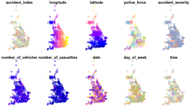
(691,641) rows (crash points), with 31 columns (see Lovelaceet al. 2019 for details on the data). This is easy to work with in-memory on modern computers, though consumes 1/3 GB of RAM. These can be converted into a spatial class, defined by the sf package (Pebesma 2018). A sample of 1000 records is taken and plotted, for demonstration purposes, as follows (see the resulting Figure 1):
a_sf = format_sf(a)
a_sample = a_sf %>% sample_n(1000)
plot(a_sample)
Having gained a measure of the crash data, and some key descriptive
statistics, we can proceed to join-on the associated casualty and
vehicle tables. The following command uses the argument type to
specify which table from the STATS19 schema is to be read-in:
c = map_dfr(y, get_stats19, type = "casualties")
v = map_dfr(y, get_stats19, type = "vehicle")
We are interested in accidents in which a pedestrian was injured and where the (only) vehicle involved was a car. This subset of the casualties dataset can be extracted as follows:
c_ped = c %>% filter(casualty_type == "Pedestrian")
v_car = v %>% filter(vehicle_type == "Car")
a_cp = a_sf %>%
  filter(number_of_vehicles == 1 & number_of_casualties == 1) %>%
  filter(accident_index %in% c_ped$accident_index) %>%
  filter(accident_index %in% v_car$accident_index)
Before proceeding, we join the vehicle and crash tables onto the crash data as follows, to create the main input dataset used in this paper:
a_cpj = a_cp %>%
  inner_join(v_car) %>%
  inner_join(c_ped)
The resulting dataset, a_cpj, contains 78,454 rows: 11% of the crashes
in the original dataset represent a car-pedestrian collision involving a
single vehicle and a single casualty (the pedestrian). This dataset,
which contains 68 columns, will be used for the remainder of this
analysis, and can be downloaded from the paper’s GitHub repo and loaded
as
follows:
u = "https://github.com/Robinlovelace/stats19-gisruk/releases/download/0.0.1/a_cpj.Rds"
download.file(url = u, destfile = "a_cpj.Rds")
a_cpj = readRDS("a_cpj.Rds")
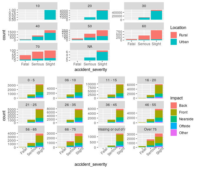
The final code chunk in this section generates plots that expose insight into the nature of car-pedestrian crashes. As illustrated in Figures 2 and 3, the results match prior expectations: elderly people (in the 66-75 and 75+ age bands) and fast roads (40 to 70 miles per hour) tend to result in more serious and fatal injuries.
g = ggplot(a_cpj)g + geom_bar(aes(accident_severity, fill = urban_or_rural_area)) +
facet_wrap(vars(speed_limit), scales = "free_y") +
labs(fill = "Location")
g + geom_bar(aes(accident_severity, fill = impact)) +
facet_wrap(vars(age_band_of_casualty), scales = "free_y") +
theme(axis.text.x = element_text(angle = 45))The data is still in a spatial form, of class sf, enabling geographic
analysis. Although the geographic resolution of the data is high, ~10 m,
we will analyse it at the national level, to investigate the relative
performance of different police forces over time. A geographic join will
be used to assign a police force to each crash (although police force is
already a variable in the dataset):
agg_slight = aggregate(a_cpj["accident_severity"], police_boundaries,
                      function(x) sum(grepl(pattern = "Slight", x)))
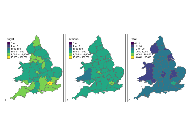
Repeating this process for each crash severity type results in the plot presented in Figure 3. Because a log scale is used between the different crash categories, the results shown in Figure 3 shows that, outside London, serious and fatal crashes are comparatively common in some areas. We can identify which police forces have the highest ratios of crashes that are reported as fatal. The top 5 and bottom 5 are shown in Table 1, which shows wide variability. As would be expected, large cities (where average speeds tend to be low) tend to have a relatively low percentage of car-pedestrian casualties that are fatal, whereas predominantly rural forces such as Wiltshire and Gloucestershire (where the roads tend to be faster, and there are fewer crashes overall) have a relatively high proportion that are fatal. Devon and Cornwall is an outlier: a relatively rural force with a low proportion of fatalities. Further research could seek to explore the reasons for this variability.
| name | slight | serious | fatal | percent_fatal |
|---|---|---|---|---|
| Wiltshire | 428 | 155 | 15 | 2.5 |
| Gloucestershire | 347 | 137 | 10 | 2.0 |
| West Mercia | 772 | 216 | 20 | 2.0 |
| Northamptonshire | 515 | 187 | 14 | 2.0 |
| Suffolk | 546 | 116 | 13 | 1.9 |
| NA | NA | NA | NA | NA |
| Devon and Cornwall | 1556 | 384 | 16 | 0.8 |
| Lancashire | 1718 | 626 | 19 | 0.8 |
| Nottinghamshire | 1102 | 290 | 10 | 0.7 |
| Metropolitan Police | 13552 | 2303 | 109 | 0.7 |
| City of London | 69 | 21 | 0 | 0.0 |
Top and bottom 5 police forces in terms of the percentage of car-pedestrian crashes that are fatal.
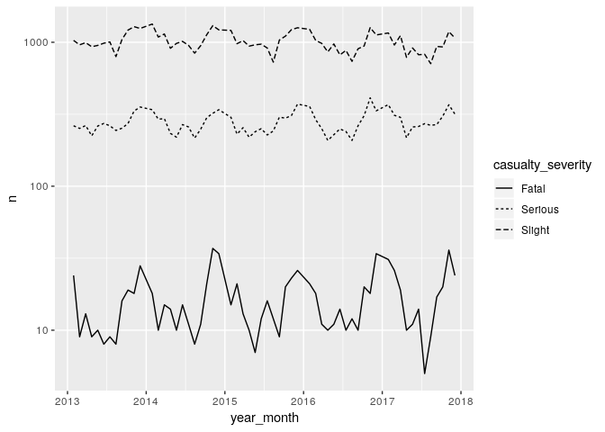
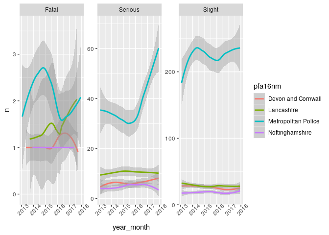
What about variability over time? The overall trend in the number of pestrians hit by cars can be seen in Figure 4, which shows the total number of people by month, broken-down by crash severity. This result shows that pedestrian casualty rates have essentially flat-lined over the past 5 years, after decades of improvement. What the data does not show, however, is the geographic breakdown of these trends.
A geographic join can assign each crash to a police authority as follows:
a_cps = st_join(a_cpj, police_boundaries)The new object has the variable pfa16nm, the police force name, which
can be subsequently aggregated and then joined back onto the geographic
variable of police_boundaries. Before we plot the ‘best’ and ‘worst’
performers geographically, it is worth investigating the temporal trend
of the top and bottom forces in terms of the percentage of casualties
that were fatal (see Table 1). When disaggregated by force area (Figure
5), the incidence of fatalities is too low for reliable analysis over
time. However, the results suggest that London (controlled by the
Metropolitan Police) has seen an increase in serious, and to a lesser
extent slight, pedestrian casualties since around the beginning of 2016.
These raise the question: why? Rather than answer this question, the final analysis will explore the geographic distribution of improving/worsening performance by force area using geographically arranged small multiples (Tufte 1983).
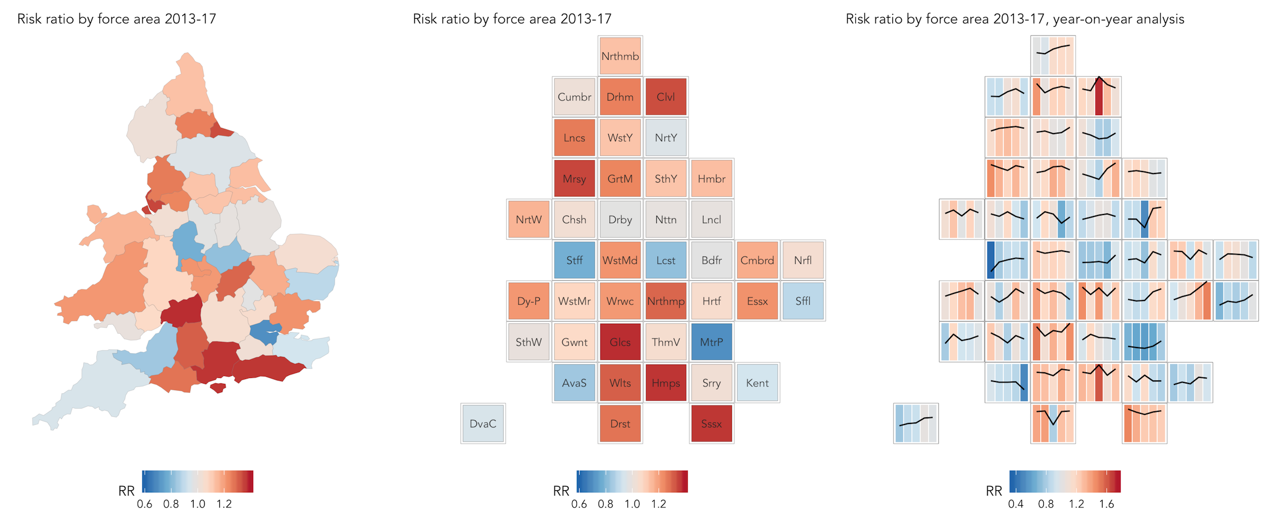
We have identified some challenges associated with disaggregate analysis of casualty data: the substantial between-force differences in absolute casualty numbers and the problem of reliably identifying temporal patterns in low incidence events such as fatalities. One measure that might allow traction on the relative severity of accidents occuring in force areas is the killed and seriously-injured rate (KSI rate) – the number of casualties that involved a fatality or serious injury as a proportion of all casualties. Analysing year-on-year change in KSI rates over the 5-year period, there appears to be a slight recent upward trend: from (0.22) in 2013-2015, to (0.23) in 2016 and (0.25) in 2017. A principled way of exploring the extent to which particular force areas are over- or under- represented in their KSI rates is by calculating risk ratios for each force ((RR_{f})), expressing the KSI rate for the force ((ksi_f)) as a ratio of the national KSI rate ((ksi_{nat})): (RR_f=ksi_f/ksi_{nat}), where a value (>1.0) indicates a higher KSI rate than nationally and a value (<1.0) indicates a KSI rate lower than the national average rate. In order to analyse year-on-year change in these force-level risk ratios and the raw KSI rates, we generate sets of small multiple charts per force, arranged according to their approximate geographic position (e.g. Figure 6) using the layout algorithm published in Meulemans et al. (2017). The first two maps in Figure 7 are choropleth maps displaying a single risk ratio statistic representing all 5 years of data; the final map supports year-on-year comparison by representing raw KSI rates as a line, with risk-ratios for each year as coloured bars.
This paper has provided a taster of what is possible with open road crash data, using packages such as stats19, revealing regional differences in the numbers, proportions and trends of one particular type of road crash: car-pedestrian collisions. However, much more is possible with the approach. A key priority in road safety research is to identify suitable denominators of risk, something that geographical methods are well-suited to answering. With new data sources, could denominators be produced at high levels of geographic resolution than the coarse Local Authority levels used in a previous studies (Lovelace, Roberts, and Kellar 2016)? More specifically, why have there been increases in serious and fatal casualties in some areas, as shown in the previous section? This finding is concerning, especially in the context of the government’s commitment to contribute to the European Union’s target of halving road traffic deaths by 2050,[2] and recent concerns from road safety advocates about recent trends in road traffic deaths.[3]
The richness of road crash data means that it can be disaggregated in many ways, beyond the results presented in this paper: there are 50+ columns and hundreds of thousands of roads represented in the joined STATS19 data, suggesting future research questions, including:
- What kinds of places have seen improvements in road safety, and how can we learn from these?
- Can automated summary graphics provide insight into performance and early warnings of increases in certain types of crashes?
- And can recent findings about the effectiveness of different interventions, particuarly around 20 mph zones and limits (Grundy et al. 2009; Aldred et al. 2018) be replicated using open data and publicly available code?
From a GIS perspective, the data presented in this paper are of interest in terms of their size (there are several million points in the open STATS19 data, going back to 1979), richness and spatial resolution (in the order of 10m, but how accurate are the coordinates?). One area where geographic research can help is in data visualisation, with new packages such as geoplumber opening the possibility of open source web applications, building on sites such as www.crashmap.co.uk and www.pct.bike to inform policy and public debate (Lovelace et al. 2017). More theoretical directions are suggested by the complex processes underlying crash data (point patterns on a linear network). But while so many people die on the roads each year in the UK (1,793 people in 2017, 3 deaths per 100,000) and worldwide (1,250,000 people in 2015, 17 deaths per 100,000) and ‘vision zero’ remains a Swedish dream (Johansson 2009), we urge people researching STATS19 and other road safety datasets to focus on a more urgent question: how to stop this carnage?
The work was funded by the Leeds Insititute for Transport Studies (ITS) Consumer Data Resarch Center (CDRC) at Leeds Institute for Data Analytics (LIDA). Thanks to open source software developers who made all this possbile, and to GitHub, where the source code behind this paper is hosted: https://github.com/Robinlovelace/stats19-gisruk
Aldred, Rachel, Anna Goodman, John Gulliver, and James Woodcock. 2018. “Cycling Injury Risk in London: A Case-Control Study Exploring the Impact of Cycle Volumes, Motor Vehicle Volumes, and Road Characteristics Including Speed Limits.” Accident Analysis & Prevention 117 (August): 75–84. https://doi.org/10.1016/j.aap.2018.03.003.
Bonney, Rick, Jennifer L. Shirk, Tina B. Phillips, Andrea Wiggins, Heidi L. Ballard, Abraham J. Miller-Rushing, and Julia K. Parrish. 2014. “Next Steps for Citizen Science.” Science 343 (6178): 1436–7. https://doi.org/10.1126/science.1251554.
Department for Transport. 2017. “Road Safety Data.”
Elvik, Rune, Truls Vaa, Alena Erke, and Michael Sorensen. 2009. The Handbook of Road Safety Measures. Emerald Group Publishing.
Grundy, Chris, Rebecca Steinbach, Phil Edwards, Judith Green, Ben Armstrong, and Paul Wilkinson. 2009. “Effect of 20 Mph Traffic Speed Zones on Road Injuries in London, 1986-2006: Controlled Interrupted Time Series Analysis.” BMJ 339 (December): b4469. https://doi.org/10.1136/bmj.b4469.
Johansson, Roger. 2009. “Vision Zero a Policy for Traffic Safety.” Safety Science, Occupational Accidents and Safety: The Challenge of Globalization / Resolving multiple criteria in decision-making involving risk of accidental loss, 47 (6): 826–31. https://doi.org/10.1016/j.ssci.2008.10.023.
Kim, Karl, and Ned Levine. 1996. “Using GIS to Improve Highway Safety.” Computers, Environment and Urban Systems 20 (4-5): 289–302.
Lovelace, Robin, Anna Goodman, Rachel Aldred, Nikolai Berkoff, Ali Abbas, and James Woodcock. 2017. “The Propensity to Cycle Tool: An Open Source Online System for Sustainable Transport Planning.” Journal of Transport and Land Use 10 (1). https://doi.org/10.5198/jtlu.2016.862.
Lovelace, Robin, Malcolm Morgan, Layik Hama, and Mark Padgham. 2019. “Stats19: A Package for Working with Open Road Crash Data.” Journal of Open Source Software. https://doi.org/10.21105/joss.01181.
Lovelace, Robin, Jakub Nowosad, and Jannes Meunchow. 2019. Geocomputation with R. CRC Press.
Lovelace, Robin, Hannah Roberts, and Ian Kellar. 2016. “Who, Where, When: The Demographic and Geographic Distribution of Bicycle Crashes in West Yorkshire.” Transportation Research Part F: Traffic Psychology and Behaviour, Bicycling and bicycle safety, 41, Part B. https://doi.org/10.1016/j.trf.2015.02.010.
Meulemans, W., J. Dykes, A. Slingsby, C. Turkay, and J. Wood. 2017. “Small Multiples with Gaps.” IEEE Transactions on Visualization & Computer Graphics 23 (1): 381–90.
Pebesma, Edzer. 2018. “Simple Features for R: Standardized Support for Spatial Vector Data.” The R Journal.
Peled, Ammatzia, and A. Shalom Hakkert. 1993. “A PC-Oriented GIS Application for Road Safety Analysis and Management.” Traffic Engineering & Control 34 (8).
Razzak, Junsid, Uzma R. Khan, and Sabeena Jalal. 2011. “Application of Geographical Information System (GIS) for Mapping Road Traffic Injuries Using Existing Source of Data in Karachi, Pakistana Pilot Study.” Journal of the Pakistan Medical Association 61 (7): 640.
R Core Team. 2019. “R: A Language and Environment for Statistical Computing.” Vienna, Austria: R Foundation for Statistical Computing.
Steenberghen, Thérèse, T. Dufays, Isabelle Thomas, and Benoît Flahaut. 2004. “Intra-Urban Location and Clustering of Road Accidents Using GIS: A Belgian Example.” International Journal of Geographical Information Science 18 (2): 169–81.
Tufte, E. 1983. Visual Display of Quantitative Information. Cheshire, CT, USA: Graphics Press.
Vicente-Saez, Ruben, and Clara Martinez-Fuentes. 2018. “Open Science Now: A Systematic Literature Review for an Integrated Definition.” Journal of Business Research 88 (July): 428–36. https://doi.org/10.1016/j.jbusres.2017.12.043.
Xie, Yihui, J. J. Allaire, and Garrett Grolemund. 2018. R Markdown: The Definitive Guide. 1 edition. Boca Raton: Chapman and Hall/CRC.
-
Note: the following code chunks are time-consuming and require interactive use of R to run. To save time, we recommend that people who want to reproduce the results start by downloading the clean
a_cpjdataset. This can be found, alongside other datasets generated for this paper, at github.com/Robinlovelace/stats19-gisruk. Code to download this dataset is provided below, in the code chunk that contails the functiondownload.file()to download the pre-processed dataset. -
https://fleetworld.co.uk/uk-falling-behind-on-road-safety-targets/
-
http:https://www.brake.org.uk/facts-resources/1653-uk-road-casualties
