The goals / steps of this project are the following:
- Load the data set (see below for links to the project data set)
- Explore, summarize and visualize the data set
- Design, train and test a model architecture
- Use the model to make predictions on new images
- Analyze the softmax probabilities of the new images
- Summarize the results with a written report
- Download the data set. The classroom has a link to the data set in the "Project Instructions" content. This is a pickled dataset in which we've already resized the images to 32x32. It contains a training, validation and test set.
- Clone the project, which contains the Ipython notebook and the writeup template.
git clone https://github.com/udacity/CarND-Traffic-Sign-Classifier-Project
cd CarND-Traffic-Sign-Classifier-Project
jupyter notebook Traffic_Sign_Classifier.ipynbI used numpy and the pandas library to calculate summary statistics of the traffic signs data set:
- The size of training set is 34799
- The size of the validation set is 4410
- The size of test set is 12630
- The shape of a traffic sign image is (32, 32, 3)
- The number of unique classes/labels in the data set is 43
Here is an exploratory visualization of the data set. First, I made sure that data is loaded correctly and all datasets
contain valid traffic sign images:
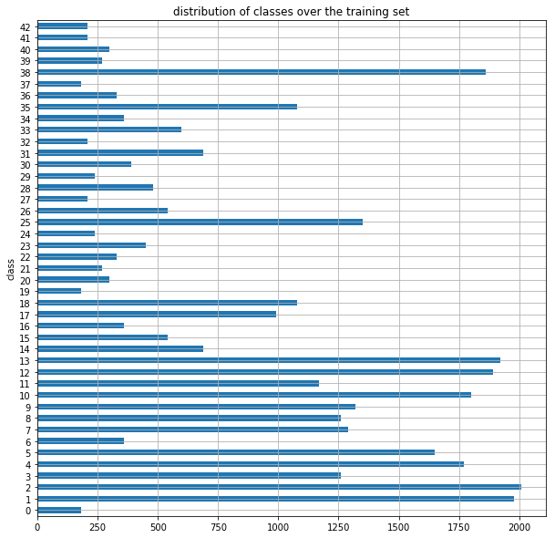
The following bar chart displays the distribution of the classes in the training set:
Outlined above, the training dataset is not balanced across classes. In fact, the classes with the most samples contain about 10 times more data than the classes with the least amount of samples. In order to improve the accuracy of the neural network, this could be addressed by using oversampling techniques like SMOTE.
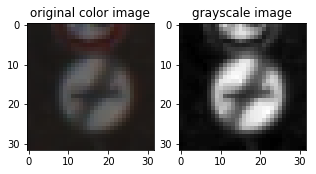
As a first step, I decided to convert the images to grayscale because it leads to higher accuracy than RGB colors on my model what I have derived from testing both approaches. Here is an example of a traffic sign image before and after grayscaling:
Furthermore, I have normalized the grayscale images. For that, the OpenCV-function cv2.normalize() has proven to be
the best choice as it provides high performance and reaches approximately zero mean.
The mean over the entire set of training images has been around 82.6776 before and around 0.0159 after normalization.
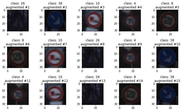
Finally, I decided to generate additional images for training because the original dataset of 34799 images is susceptible for overfitting. To train for a few more epochs without overfitting my network, I used data augmentation techniques provided through the Keras module of TensorFlow. In particular, I shifted the images within a range of (-2, 2) in width and height, used a random zoom factor between 0.9 and 1.1 and rotated them between -15 and +15 degrees.
The following picture shows an example of a reduced batch of five images from the original dataset:
In the next figure three batches of random augmentations of these images are illustrated:
The augmented set multiplies the count of original training images by 6 which leads to 34799 * 6 = 208794 images that include both, the original and augmented images.
My final model consists of the following layers:
| Layer | Description |
|---|---|
| Input | 32x32x1 grayscale image |
| Convolution 5x5 | 1x1 stride, valid padding, outputs 28x28x6 |
| RELU | |
| Max pooling | 2x2 stride, outputs 14x14x6 |
| Convolution 5x5 | 1x1 stride, valid padding, outputs 10x10x16 |
| RELU | |
| Max pooling | 2x2 stride, outputs 5x5x16 |
| Flatten | outputs 400 |
| Fully connected | outputs 120 |
| RELU | |
| Dropout | dropout probability 50% |
| Fully connected | outputs 84 |
| RELU | |
| Dropout | dropout probability 50% |
| Fully connected | outputs 43 |
To train the model, I used a batch size of 32 and trained the model for 8 epochs in total. Biases are initialized to zero and weights are initialized to a truncated normal distribution. Learning is done via the AdamOptimizer with a rate of 0.001 at the beginning. Learning rate decay and momentum is set to TensorFlow's default values for that optimizer. As a loss function I used softmax cross entropy loss.
My final model results were:
- training set accuracy of 91.0% (with dropout)
- validation set accuracy of 96.6%
- test set accuracy of 94.7%
First off, I started building a model with the LeNet-architecture as described by Yann LeCun in "Gradient-Based Learning Applied to Document Recognition". My plan behind this was to use a simple architecture that works efficient enough on systems with limited resources, reaches sufficient accuracy on smaller datasets and is easy to fiddle with for a less experienced machine learning engineer. Then, I wanted to keep the structure of the layers and tried to use other techniques to improve the accuracy. Additionally, I used TensorBoard for logging the training and validation accuracy and loss to keep track of iterative improvements and compare performance of different hyperparameters.
So, the first thing I tweaked was the normalization of images. Normalizing each image simply by (pixel - 128) / 128
for each pixel still led to a significantly higher mean than zero. After trying out (pixel - 255) / 255 which should
lead to color values between (0.0, 1.0) that reduced the mean a bit further, I looked for library functions to
accomplish an even better normalization. One way would have been to use numpy's functions like numpy.amax() to get
the maximum color value of the image and scale it to 1.0 and scale all other values by the same factor. However, I
tried OpenCV's function cv2.normalize() which performed faster than the previous solution and finally resulted in a
mean of 0.0159.
Next, I observed that the model starts to overfit after just a few epochs (validation loss suddenly increasing while training loss is still decreasing) which is plausible as our dataset only contains around 35,000 images for training 43 different classes. So, the most effective way to address overfitting appeared to be increasing the amount of available data by using data augmentation. See Pre-process the image data (1) for final parameters and examples. I took into account that the used augmentation methods do not affect the semantics of the traffic sign (e.g. flipping is not suitable as speed limits would become mirrored).
Moreover, I applied dropout with a probability of 50% after the fully connected layers to reduce overfitting. This allowed me to train for more epochs without overfitting, leading to higher accuracy in the end. Although, Park & Kwak have described in chapter 3 "Effectiveness of Dropout in Convolutional Layer" in their paper that a dropout of 10% applied after a convolutional layer can improve accuracy, I did not achieve better results with it. Therefore, I did not add it to the final model. Testing different probabilities of 10%, 20%, 40%, 50%, 60%, 80% and 90% has turned out that dropout of 50% only after the fully connected layers reaches the best accuracy here.
In the following, I decided to determine the initial learning rate of the model. From 1e-2, 1e-3 and 1e-4 as rates, 1e-3 performed the best. 1e-4 learns too slow on a relatively small dataset and 1e-2 is too high and results in overfitting again. Learning rate decay is handled by the default parameters of TensorFlow for the AdamOptimizer.
Furthermore, I considered other initialization methods for the biases and weights of layers. Ganegedara suggests using Xavier initialization for weights. However, it showed little to no effect as opposed to truncated normal initialization in the final accuracy. Initializing the biases to a small constant value instead of setting them to zero also made no significant difference.
Another modification to my network was to allow creating a model with either grayscale or RGB images.
The following screenshot sketches the evaluation process of different models in TensorBoard. It features models with normal and Xavier initialization and colorspaces of either RGB or grayscale:
Last but not least, I found out that more regularization using L2 loss leads to worse results for this network which might be an effect of too much regularization on a rather small dataset size.
Further additions to improve accuracy could include model ensembles, different network architectures, transfer learning and balancing the dataset in terms of class distribution which are beyond the scope of this work for now.
Here are five German traffic signs that I found on the web:
The first image might be difficult to classify because the contrast of the red sign to the red roof in the background is rather small and on the back side of the sign there is another sign for traffic in the opposite direction. So, it could be an issue that the different shape of the two signs may not be distinguished.
The second image has a stronger motion blur and a small noisy point in the middle of the image which might lead to difficulties.
The third image might be difficult to classify because the sun reflects on the sign in the lower left corner. This corner holds an important part of the signs' features.
The fourth image might be difficult to classify because it is a sign with relatively low contrast in general as it is only gray and black. Gray might often be perceived as unimportant background features by human eyes. Also, this class has one of the least amount of samples in the training set.
The last image has been taken during rainy conditions. The right half of the sign is affected by a raindrop and therefore distorts this area of the image which might lead to difficulties.
Here are the results of the prediction:
| Image | Prediction |
|---|---|
| No entry | No entry |
| Bumpy road | Bumpy road |
| Slippery road | Slippery road |
| End of all speed and passing limits | Yield |
| Ahead only | Ahead only |
The model was able to correctly guess 4 of the 5 traffic signs, which gives an accuracy of 80%. If compared to the accuracy on the test set of 94.7%, these predictions perform worse.
The final model for making predictions is created at the end of "Train, Validate and Test the Model" of the IPython notebook and the predictions are called at "Predict the Sign Type for Each Image". The code of the model including the process of getting the prediction probabilities is located in the class TrafficSignNetwork of the notebook.
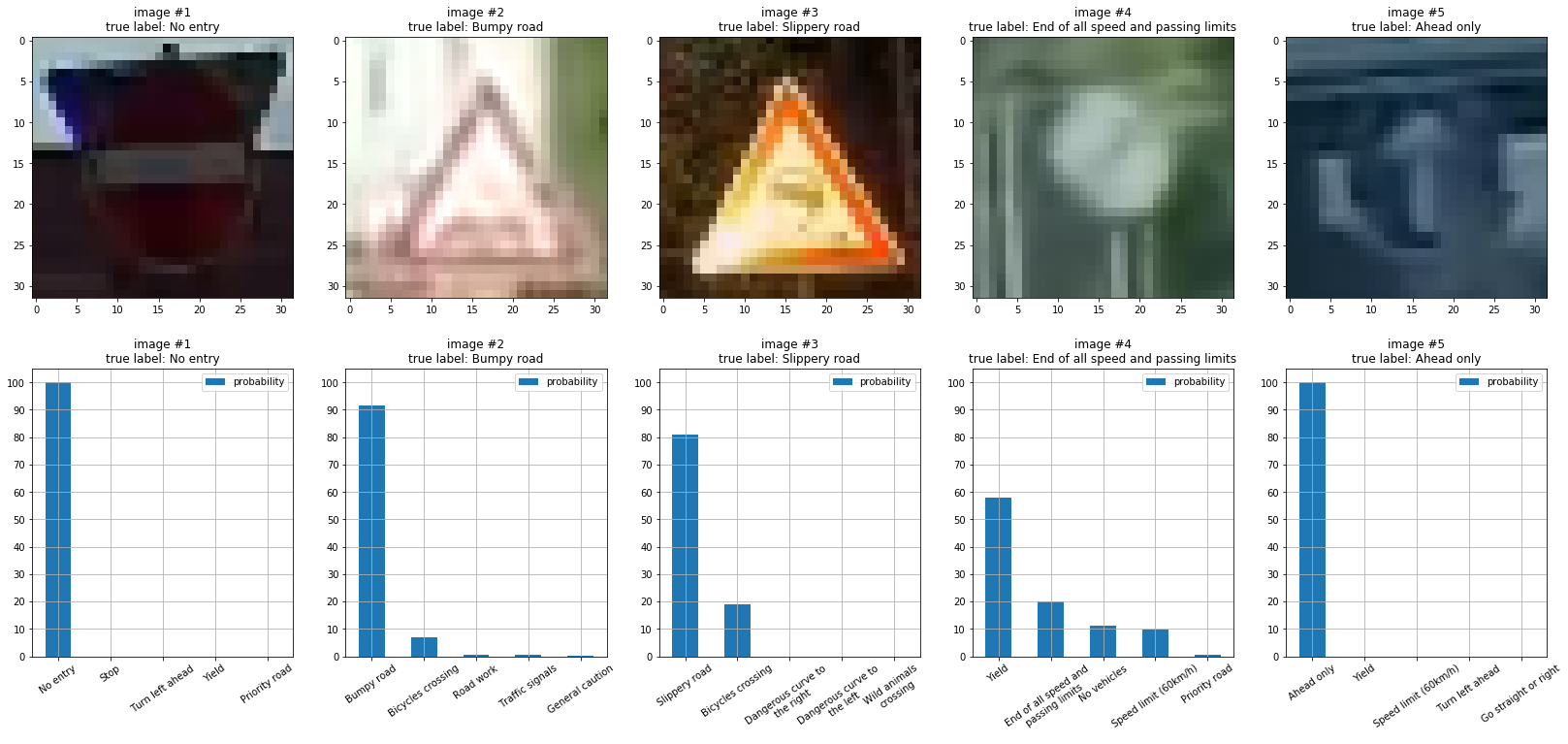
The following diagram visualizes the top 5 softmax probabilities of each image:
The model is almost 100% certain about the prediction of the first and last image.
On the second image, the model is also relative sure about the prediction with a probability of over 90%.
The third image shows a slightly lower probability of about 80% but this can still be considered a high value.
Lastly, the fourth image is predicted wrong. "Yield" has the highest probability with almost 60% and the correct labels prediction comes second with only 20%. This corresponds to the observations I made earlier that this sign might be hard to classify. The network might need more samples for this class to recognize them better.
In my opinion, it shows some interesting results. The trained network picks up edges and specific details of the sign. I think it especially picks up those borders which often reflect the light stronger through the contrast of colors and special material leading to those reflections. Moreover, it seems that especially feature map 0 and 2 recognized the indicator for a bumpy road at the bottom of the sign.
However, two filters (FeatureMap 1 and FeatureMap 4) do not activate at all which we could examine further and find out for which types of images it would activate. But, that is beyond the scope of this project.


