Table of Contents

Machine Learning systems today aid decision making across the entire spectrum of life. One such decision, that each human has to make daily is his/her "meal choice" . The said decision depends on a multitude of factors like nutritional requirements, eating preferences and mood etc.
In this project, we thus aim to build an ML system that aids multiple aspects of Meal Choice decision using Image Recognition and Recommender Systems.
We want to tackle two main problems here:
-
Given an image of a food item, what are the key ingredients that goes in preparing the food item ?
-
What food items should we recommend to a user based on his preferences and other similar users food choices?
- Can the recommendation also account for additional constraints from user like nutritional requirements, calories level, etc?
The modular nature of above problems lends itself to multiple usecases:
-
When encountered with an unknown food item, the user might want to know its ingredients, such that he can figure out:
- Is the dish healthy?
- If the dish contains allergens?
-
As a next step, user might want recommendations for similar dishes that he took image of. Additionally, there can be numerous additional constraints placed on the recommendations recieved like:
- Restrict recommendations to ingredients he already has
- Constrain by the nutritional requirements of the dish, say the user wants only "low calorie" dishes.
We divide our project pipeline into three main stages:
-
Classfication System: This stage would take as input food images and passes them through a CNN to output food labels. The output of this stage is (Output 1), and flows to next stage, but can also be used independently.
-
Food to Ingredient Mapping: Output 1 from CNN is then queried through a database housing the mapping between food items and their respective ingredients, to yield Output 2. This can again either be used independently or overlaid over recommendation system as a filter.
-
Recommendation System: In this stage we reccommend the user additional food items: Output 3 basis his (&other individuals) interactions. We also allow for the user to place additional constraints over the recommendations.
The schematic of these stages is given below:

We will be using Food-101 dataset for the CNN classification which consists of 101 food categories with a total of 101,000 images.
In this part, we’re using data from the Food.com Recipes and Interactions, which contains 2 datasets: user interactions data and recipe dataset
- user interactions dataset: This dataset contains the user Id and users’ interaction with recipes, such as rating and review.
- recipe dataset: This dataset contains the recipe information recipe ID, nutrition information, steps to cook, time to cook, etc.
We will join user interactions dataset and recipe dataset based on recipe_id. With the joined data, we’ll use our recommendation system to study user preferences and recommend recipes to users based on their previous behaviors, and optionally input from the ingredient we get from the classification task.
As defined in the pipeline above, there are three main modules of our ML system, and this section details the results and discussion of the work done until now on each of the items.
In this module, we have trained a CNN model to predict the correct food category out of 101 classes using a pretrained resnet34 and resnet50 architecture. We are using fastai deep learning library to create the pipeline for the model
For each category, we have 750 images in the training set and 250 images in the test set. The training set is split into 20% validation and 80% training set.
Total Training set: 60600 images
Total Validation set: 15150 images
Total Test set: 25250 images

Scatterplot for the image sizes reveals that images are not of the same size. This can cause irregularities in our training. We will need to transform the images and make the dataset of the same size to maintain conistency while training.
To tackle this problem, all the images have been resized to 224x224 so that each image sample has the same matrix size while training the data.
A sample can be seen below for the dataset.

train_data = ImageDataLoaders.from_df(df=train_df, path=path_images, fn_col=1, label_col=0, valid_pct=0.2, bs=batch_size, item_tfms=Resize(224), device=torch.device('cuda'))Training data has also been augmented with random transformations like crops, rotate, zoom, brightness and contrast to increase the sample size for the CNN models. At the same time, it also helps the model generalize better with more variance in the images.
We are using Error Rate, Top-1 accuracy and Top-5 accuracy as our metrics to compare between model performances.
Our loss function is cross-entropy.
We have used FastAI library to find the optimal learning rate. It trains learner over a few iterations. Start with a very low start_lr and change it at each mini-batch until it reaches a very high end_lr. Output will be recorded as the loss at each iteration. Plot those losses against the learning rate to find the optimal value before it diverges.
The optimal learning rate is around 1e-2, right before the minimm loss.

learn = vision_learner(train_data_aug, resnet50, metrics=[accuracy, top_5_accuracy, error_rate])
learn.lr_find()In the initial model we are leveraging transfer learning and using ResNet34 pre-trained model for classifying food items.
We are keeping the learning rate constant (1e-2) and not using adaptive learning rate. We will also be freezing the weights of the model and not re-training the last layers.

It can be seen that this model takes arond 9 mins to train for each epoch. The training loss and validation loss both seem to go down after each iteration until it almost becomes constant. We stop the model at 8 epochs. We cn also see that the error rate decreased from 0.48 to 0.31 in 8 epochs before plateauing.

The model still does not perform great as it is not able to predict well. We can see the losses for the model in the test dataset.
Our second choice of model is again a transfer learning approach with a pre-trained ResNet50 model.
The advantage of ResNet34 vs ResNet50 is that latter uses a stack of 3 layers instead of the earlier 2. Therefore, each of the 2-layer blocks in Resnet34 was replaced with a 3-layer bottleneck block, forming the Resnet 50 architecture. This has much higher accuracy than the 34-layer ResNet model.
We are again keeping the learning rate constant (1e-2) and not using adaptive learning rate. We will also be freezing the weights of the model and not re-training the last layers.

This model takes an average of 13 mins to train as suggested by 16 extra layers in the model. We can observe that the model has achieves a much lower error rate in 8 epochs and we are able to achieve 73% accuracy with Top-5 accuracy of 91%.

As we can see from the graph below for Loss Vs Iterations that we are achieving a constant decrease in loss as the iteration increase and it becomes almost constant at the end.
We can also observe that there is no overfitting and training and validation losses are decreasing simultaneously. It is good to see that fitting to both the real and random patterns very well and able to classify test dataset quite well.

This model performs much better than the previous model and accurately predicts the test dataset as can be seen from the sample.

The model's top losses can be seen here where it predicts with quite high possibility but misclassifies.
Unfreezing the model
We can unfreeze the CNN layers of the model and train the weights along with the fully connected layers to improve the accuracy of our model.


As we can see we were able to increase the overall accuracy to 79.8% and the top-5 accuracy to 94% for our model.
- Exploring different architectures such as ResNet200 and Efficient Net to train the model and check for increase in accuracy.
Once we have predicted the label using the above CNN module, we will map this label to our recipe dataset and extract the ingredients list. The ingredients data would then feed into the recommendation system and help to give more filtered and personalized recommendations.
Therefore, we want to match the labels generated by the CNN model and the names in the recipe table, which contains the dishes' ingredients.
In order to achieve this, we matched all the 101 labels from the Food-101 dataset to the closest recipe name in the recipe database. We used fuzzwuzzy library which calculates Levenshtein Distance between two strings to report a matching score. For every label, we used the recipe name with the highest matching score.
Below is an example of the results where every label is mapped to a recipe name and its ingredients list from the recipe database.
| label | name | id | ingredients |
|---|---|---|---|
| apple pie | apple pie | 124853 | [apple juice, raw honey, whole cloves, evercle... |
| apple pie | apple pie | 65988 | [all-purpose flour, salt, shortening, cold wat... |
| baby back ribs | baby back ribs | 502407 | [baby back ribs, orange juice, margarita mix, ... |
| baklava | baklava | 48804 | [phyllo dough, nuts, butter, ground cinnamon, ... |
| beef carpaccio | beef carpaccio | 189130 | [beef tenderloin, arugula, vinaigrette, kosher... |
To build a coherent pipeline between the CNN and the Recommendation module, we used this preprocessed output to get the ingredients list for the predicted label. Once, we have the ingredients list, we will use this as filters while recommending new recipes to the user.
Also, we are recommending recipes to a user by picking a user_id at random from the RAW_interactions.csv file.
We will use the user-food interaction data which contains the temporal food-item ratings given by users to provide recommendations for similar food items leveraging the user-user collaborative filtering and matrix factorization techniques.

The user interaction recipe data has 5 columns, with head of the table given below:
Index(['user_id', 'recipe_id', 'date', 'rating', 'review'], dtype='object')| user_id | recipe_id | date | rating | review |
|---|---|---|---|---|
| 38094 | 40893 | 2003-02-17 | 4 | Great with a salad. Cooked on top of stove for... |
| 1293707 | 40893 | 2011-12-21 | 5 | So simple, so delicious! Great for chilly fall... |
| 8937 | 44394 | 2002-12-01 | 4 | This worked very well and is EASY. I used not... |
| 126440 | 85009 | 2010-02-27 | 5 | I made the Mexican topping and took it to bunk... |
| 57222 | 85009 | 2011-10-01 | 5 | Made the cheddar bacon topping, adding a sprin... |
The number of unique users and unique recipes is given as:
user_id         226570
recipe_id       231637
user_recipe    1132367
As expected not every user rates every recipe, which is apparent from the counts above. An estimate of the sparsity of interaction matrix is:
sparsity = 1- (1132367/(N_users*N_Recipes))
print (f"Sparsity in data {sparsity:.9%}")
#Sparsity in data 99.997842371%
We have analysed the distribution of these interactions below:
- How many recipes do the users rate?
user_grp[[("recipe_id","count")]].quantile([0.1,0.2,0.3,0.4,0.5,0.6,0.7,0.8,0.9,1])| Percentile | 0.1 | 0.2 | 0.3 | 0.4 | 0.5 | 0.6 | 0.7 | 0.8 | 0.9 | 1.0 |
|---|---|---|---|---|---|---|---|---|---|---|
| recipe_id,count | 1.0 | 1.0 | 1.0 | 1.0 | 1.0 | 1.0 | 1.0 | 2.0 | 5.0 | 7671.0 |
Thus almost 90% of the users rate <=5 recipes, to create a heavy left tail skew.
- How many users rate the same recipes ? The converse of the above distribution is the distribution of users rating the same recipe.
recipe_grp[[("user_id","count")]].quantile([0.1,0.2,0.3,0.4,0.5,0.6,0.7,0.8,0.9,1])| Percentile | 0.1 | 0.2 | 0.3 | 0.4 | 0.5 | 0.6 | 0.7 | 0.8 | 0.9 | 1.0 |
|---|---|---|---|---|---|---|---|---|---|---|
| user_id,count | 1.0 | 1.0 | 1.0 | 2.0 | 2.0 | 3.0 | 3.0 | 5.0 | 9.0 | 1613.0 |
Similar to above we see a highly skewed distribution, with 80% of the recipes being rated by <=5 users
- Distribution of Ratings?
raw_interactions["rating"].hist()
The ratings follow a heavy skew, with 4 and 5 being the predominant rating
The recipe data has 12 columns and 231636 rows, which gives us 231636 unique recipes with 12 features.
Index(['name', 'id', 'minutes', 'contributor_id', 'submitted', 'tags',
       'nutrition', 'n_steps', 'steps', 'description', 'ingredients',
       'n_ingredients'],
      dtype='object')
Among the 231636 recipes, there is only one data point that is a missing value. The data point doesn't have attribute name. Therefore, we delete this datapoint.
After analyzing the quantitative data, we found that the mean steps of cooking is around 9.5 steps; mean cooking time is about 9 mins, and mean number of ingredient is around 9. Also, there is positive relations between steps and ingredients.
The distribution of few features in metadata is given below:
| minutes | n_steps | n_ingredients | |
|---|---|---|---|
| count | 2.316360e+05 | 231636.000000 | 231636.000000 |
| mean | 9.398587e+03 | 9.765516 | 9.051149 |
| std | 4.461973e+06 | 5.995136 | 3.734803 |
| min | 0.000000e+00 | 0.000000 | 1.000000 |
| 25% | 2.000000e+01 | 6.000000 | 6.000000 |
| 50% | 4.000000e+01 | 9.000000 | 9.000000 |
| 75% | 6.500000e+01 | 12.000000 | 11.000000 |
| max | 2.147484e+09 | 145.000000 | 43.000000 |
The n_ingredient data is skew to the right, however, the mode of n_ingredients is also around 9 and 10.

The correlation between few important metadata features are given below:
| minutes | n_steps | n_ingredients | |
|---|---|---|---|
| minutes | 1.000000 | -0.000257 | -0.000592 |
| n_steps | -0.000257 | 1.000000 | 0.427706 |
| n_ingredients | -0.000592 | 0.427706 | 1.000000 |
Also the minutes column has a lot of very high noisey values, so we have capped the variable to 48*60 or (48 hrs * 60 minutes).
The metadata above lends to few intuitive hypotheses, like are more complex dishes rated lower? We have performed Hypothesis testing for this, and this helps us to tune our models.
Effect of Minutes required to cook on the rating of the dish We have bucketed the cleaned minutes variable into meaningful buckets, which is then used to analyse the effect on other variables.
| minutes_buckets | n_ingredients | n_steps | rating |
|---|---|---|---|
| a.<=15 | 6.503086 | 5.737489 | 4.469096 |
| b.<=30 | 8.597985 | 8.877021 | 4.427940 |
| c.<=60 | 9.607273 | 10.610071 | 4.405543 |
| d.<=240 | 10.337944 | 12.156324 | 4.383287 |
| e.>240 | 9.147623 | 9.792240 | 4.310574 |
As expected, with increasing number of buckets, the average rating decreases, while number of steps and number of ingredients increase. There might be a intrinsic bias in this trend, as people investing more time in the cooking, might generally have a higher standard set for rating too.

We have also performed Pair wise ANOVA (Tukey) test to ascertain the same.
from statsmodels.stats.multicomp import pairwise_tukeyhsd
def ad_tukey(grp="",reponse=""):
    tukey = pairwise_tukeyhsd(endog=joined_df[response],
                          groups=joined_df[grp],alpha=0.01)
    print (tukey)

# perform Tukey's test
grp = "minutes_buckets"
for response in ["rating","n_ingredients", "n_steps"]:
    print (f"Group Variable: {grp}, Response Variable: {response}")
    ad_tukey(grp,response)
    print()
Group Variable: minutes_buckets, Response Variable: rating
Multiple Comparison of Means - Tukey HSD, FWER=0.01
=====================================================
group1 group2 meandiff p-adj lower upper reject
-----------------------------------------------------
a.<=15 b.<=30 -0.0412 0.0 -0.0533 -0.029 True
a.<=15 c.<=60 -0.0636 0.0 -0.0751 -0.052 True
a.<=15 d.<=240 -0.0858 0.0 -0.0982 -0.0735 True
a.<=15 e.>240 -0.1585 0.0 -0.1763 -0.1407 True
b.<=30 c.<=60 -0.0224 0.0 -0.033 -0.0118 True
b.<=30 d.<=240 -0.0447 0.0 -0.0561 -0.0332 True
b.<=30 e.>240 -0.1174 0.0 -0.1345 -0.1002 True
c.<=60 d.<=240 -0.0223 0.0 -0.0331 -0.0114 True
c.<=60 e.>240 -0.095 0.0 -0.1117 -0.0782 True
d.<=240 e.>240 -0.0727 0.0 -0.09 -0.0554 True
-----------------------------------------------------
Group Variable: minutes_buckets, Response Variable: n_ingredients
Multiple Comparison of Means - Tukey HSD, FWER=0.01
=====================================================
group1 group2 meandiff p-adj lower upper reject
-----------------------------------------------------
a.<=15 b.<=30 2.0949 0.0 2.0616 2.1282 True
a.<=15 c.<=60 3.1042 0.0 3.0725 3.1359 True
a.<=15 d.<=240 3.8349 0.0 3.801 3.8687 True
a.<=15 e.>240 2.6445 0.0 2.5959 2.6932 True
b.<=30 c.<=60 1.0093 0.0 0.9802 1.0383 True
b.<=30 d.<=240 1.74 0.0 1.7086 1.7713 True
b.<=30 e.>240 0.5496 0.0 0.5027 0.5966 True
c.<=60 d.<=240 0.7307 0.0 0.701 0.7603 True
c.<=60 e.>240 -0.4597 0.0 -0.5055 -0.4138 True
d.<=240 e.>240 -1.1903 0.0 -1.2377 -1.143 True
-----------------------------------------------------
Group Variable: minutes_buckets, Response Variable: n_steps
Multiple Comparison of Means - Tukey HSD, FWER=0.01
=====================================================
group1 group2 meandiff p-adj lower upper reject
-----------------------------------------------------
a.<=15 b.<=30 3.1395 0.0 3.0874 3.1917 True
a.<=15 c.<=60 4.8726 0.0 4.823 4.9222 True
a.<=15 d.<=240 6.4188 0.0 6.3659 6.4718 True
a.<=15 e.>240 4.0548 0.0 3.9786 4.1309 True
b.<=30 c.<=60 1.733 0.0 1.6875 1.7786 True
b.<=30 d.<=240 3.2793 0.0 3.2302 3.3285 True
b.<=30 e.>240 0.9152 0.0 0.8416 0.9888 True
c.<=60 d.<=240 1.5463 0.0 1.4998 1.5927 True
c.<=60 e.>240 -0.8178 0.0 -0.8896 -0.746 True
d.<=240 e.>240 -2.3641 0.0 -2.4382 -2.2899 True
-----------------------------------------------------Similar results are also calculated after bucketing n_steps
Group Variable: steps_buckets, Response Variable: rating
Multiple Comparison of Means - Tukey HSD, FWER=0.01
====================================================
group1 group2 meandiff p-adj   lower   upper  reject
----------------------------------------------------
 a.<=5 b.<=10  -0.0306    0.0 -0.0402 -0.0211   True
 a.<=5 c.<=20  -0.0402    0.0 -0.0504 -0.0299   True
 a.<=5  d.>20  -0.0997    0.0 -0.1188 -0.0806   True
b.<=10 c.<=20  -0.0095 0.0043 -0.0183 -0.0007   True
b.<=10  d.>20   -0.069    0.0 -0.0874 -0.0507   True
c.<=20  d.>20  -0.0595    0.0 -0.0782 -0.0408   True
----------------------------------------------------

Group Variable: steps_buckets, Response Variable: n_ingredients
Multiple Comparison of Means - Tukey HSD, FWER=0.01
=================================================
group1 group2 meandiff p-adj lower  upper  reject
-------------------------------------------------
 a.<=5 b.<=10   1.5406   0.0 1.5148 1.5665   True
 a.<=5 c.<=20    3.413   0.0 3.3854 3.4407   True
 a.<=5  d.>20    4.976   0.0 4.9245 5.0275   True
b.<=10 c.<=20   1.8724   0.0 1.8486 1.8962   True
b.<=10  d.>20   3.4354   0.0 3.3859 3.4849   True
c.<=20  d.>20    1.563   0.0 1.5125 1.6134   True
-------------------------------------------------

Group Variable: steps_buckets, Response Variable: minutes1
Multiple Comparison of Means - Tukey HSD, FWER=0.01
===================================================
group1 group2 meandiff p-adj  lower   upper  reject
---------------------------------------------------
 a.<=5 b.<=10  12.5713   0.0 11.0148 14.1278   True
 a.<=5 c.<=20  19.8714   0.0 18.2029 21.5398   True
 a.<=5  d.>20  98.3795   0.0 95.2769 101.482   True
b.<=10 c.<=20   7.3001   0.0  5.8663  8.7339   True
b.<=10  d.>20  85.8082   0.0 82.8252 88.7911   True
c.<=20  d.>20  78.5081   0.0 75.4653  81.551   True
---------------------------------------------------TRAIN__Validation_SIZE = 0.8
TEST_SIZE = 0.2We have split our dataset by stratifying at the level of user_id wherever possible. In cases where we are unable to divide the interactions between our train and test set in the above ratio, we randomly pick one row and place it in Train. While evaluating our model we have also filtered our data to only include users which have a high number of interactions.
We have tried two approaches for recommendation system:
We have used user-user collaborative filtering technique to predict the ratings for recipes not yet consumed by the user and use it to fork out recommendations for recipes with the highest predicted prorbability for a given user. Also , since the number of users is comparatively lesser as compared to the number of recipes , the user-user approach is computationally efficient.
Since , this method leverages the ratings from a list of closest users corresponding to each user based on their common recipes , therefore we have filtered for only those users and recipes which have atleast 10 interactions in the overall dataset.
user_ids_count = Counter(df_raw.user_id)
user_ids_keep = [i for (i,j) in user_ids_count.most_common()[::-1] if j>=5]
df_small = df_raw[(df_raw.user_id.isin(user_ids_keep))].reset_index(drop=True)
The similarity between 2 users is computed using the Pearson Correlation coefficient based on all the ratings for the common recipes. Also , only those set of users are considered as neighboring points who have atleast 5 common recipes so that our recommendation is not biased.
The ratings are centered around mean(deviations) to handle the inherent bias in user's ratings (for e.g. some users are very lenient and always rate every recipe 4 or 5 whereas there are some users who have slightly stricter in giving ratings and they give a 3 or a 2 rating to most of the recipes).
Few hyperparameters which need to be further explored are :
-> Minimum number of interactions to consider in the collaborative filtering : 10
-> Number of neighboring points to consider : 25
-> Limit (Number of recipes in common to be considered when using pearson correlation coefficient) : 5
K = 25 # number of neighbors we'd like to consider
limit = 5 # number of common recipes users must have in common in order to consider
neighbors = {} # store neighbors in this list
averages = {} # each user's average rating for later use
deviations = {} # each user's deviation for later use
SIGMA_CONST = 1e-6

for j1,i in enumerate(list(set(df_train.user_id.values))):

    recipes_i = user2recipe[i]
    recipes_i_set = set(recipes_i)

    # calculate avg and deviation
    ratings_i = { recipe:userrecipe2rating[(i, recipe)] for recipe in recipes_i }
    avg_i = np.mean(list(ratings_i.values()))
    dev_i = { recipe:(rating - avg_i) for recipe, rating in ratings_i.items() }
    dev_i_values = np.array(list(dev_i.values()))
    sigma_i = np.sqrt(dev_i_values.dot(dev_i_values))

    # save these for later use
    averages[i]=avg_i
    deviations[i]=dev_i

    sl = SortedList()

    for i1,j in enumerate(list(set(df_train.user_id.values))):
        if j!=i:
            recipes_j = user2recipe[j]
            recipes_j_set = set(recipes_j)
            common_recipes = (recipes_i_set & recipes_j_set)
            if(len(common_recipes)>limit):

                # calculate avg and deviation
                ratings_j = { recipe:userrecipe2rating[(j, recipe)] for recipe in recipes_j }
                avg_j = np.mean(list(ratings_j.values()))
                dev_j = { recipe:(rating - avg_j) for recipe, rating in ratings_j.items() }
                dev_j_values = np.array(list(dev_j.values()))
                sigma_j = np.sqrt(dev_j_values.dot(dev_j_values))

                # calculate correlation coefficient
                numerator = sum(dev_i[m]*dev_j[m] for m in common_recipes)
                denominator = ((sigma_i+SIGMA_CONST) * (sigma_j+SIGMA_CONST))
                w_ij = numerator / (denominator)
                # insert into sorted list and truncate
                # negate absolute weight, because list is sorted ascending and we get all neighbors with the highest correlation
                # maximum value (1) is "closest"
                sl.add((-(w_ij), j))
                # Putting an upper cap on the number of neighbors
                if len(sl)>K:
                    del sl[-1]
We have evaulated the model performance based on rmse and mae value after doing a train test split on stratified sample.
print('train mse:', mse(list(train_predictions.values()), list(train_targets.values())))
print('test mse:', mse(list(test_predictions.values()), list(test_targets.values())))

print('train rmse:', rmse(list(train_predictions.values()), list(train_targets.values())))
print('test rmse:', rmse(list(test_predictions.values()), list(test_targets.values())))

print('train mae:', mae(list(train_predictions.values()), list(train_targets.values())))
print('test mae:', mae(list(test_predictions.values()), list(test_targets.values())))
train mse: 0.8615178024084629
test mse: 0.9062015866125724
train rmse: 0.9281798330110728
test rmse: 0.9519462099365554
train mae: 0.522643529733127
test mae: 0.5670269049700766
We also performed a Ranking Evaluation procedure using NDCG metric .
We do not have rankings as of now in our truth data set , so we leverage cosine similarity between recipes's embedding and user's average embedding to break up recipes with the same rating into different rankings . This would enable use to calculate various Ranking based evaluation metrics such as NDCG and MAP@k as the predictions can be categorized into ranking as their values are outlayed on a continuous scale
Our embedding vector has 3 features -> Calories , Protein and Carbs.
print(f"Mean NDCG score is {np.nanmean(ndcg_list)}")0.939857
Final piece is to integrate any user into our user-recipe interaction matrix and create a recommendation function that would find the list of nearest neighbors and fork out recommendations based on the collaborative filtering technique discussed above
Attaching the code snippet below for the get_recommendations_function
def get_recipes_recommendations(i,k):
    """
    Input : i ---> user_id for which we need recommendations
            k ---> The number of recipe recommendations wanted
    Output :
            most_related_neighbors ---> a list of most related user_id's based on pearson correlation coefficient
            recommended_recipes ---> list of recommended recipes based on similar user's likings
            common_recipes_dict ---> Dictionary of neighbors and common_recipes
    """
        common_recipes_dict = {}
        recipes_i = user2recipe[i]
        recipes_i_set = set(recipes_i)

        # calculate avg and deviation
        ratings_i = {recipe: userrecipe2rating[(i, recipe)] for recipe in recipes_i}
        avg_i = np.mean(list(ratings_i.values()))
        dev_i = {recipe: (rating - avg_i) for recipe, rating in ratings_i.items()}
        dev_i_values = np.array(list(dev_i.values()))
        sigma_i = np.sqrt(dev_i_values.dot(dev_i_values))

        # save these for later use
        averages[i] = avg_i
        deviations[i] = dev_i

        sl = SortedList()
        for j in list(set(data_train_v1.user_idx.values)):
            if j != i:
                recipes_j = user2recipe[j]
                recipes_j_set = set(recipes_j)
                common_recipes = (recipes_i_set & recipes_j_set)

                if (len(common_recipes) > limit):
                    common_recipes_dict[j] = list(common_recipes)
                    ratings_j = {recipe: userrecipe2rating[(
                        j, recipe)] for recipe in recipes_j}
                    avg_j = np.mean(list(ratings_j.values()))
                    dev_j = {recipe: (rating - avg_j)
                             for recipe, rating in ratings_j.items()}
                    dev_j_values = np.array(list(dev_j.values()))
                    sigma_j = np.sqrt(dev_j_values.dot(dev_j_values))

                    # calculate correlation coefficient
                    numerator = sum(dev_i[m]*dev_j[m] for m in common_recipes)
                    denominator = ((sigma_i+SIGMA_CONST)
                                   * (sigma_j+SIGMA_CONST))
                    w_ij = numerator / (denominator)
                    # insert into sorted list and truncate
                    # negate absolute weight, because list is sorted ascending and we get all neighbors with the highest correlation
                    # maximum value (1) is "closest"
                    sl.add((-(w_ij), j))
                    # Putting an upper cap on the number of neighbors
                    if len(sl) > K:
                        del sl[-1]

        neighbors[i] = sl
        try:
            most_related_neighbors = [j for i, j in neighbors[i][:10]]
        except:
            most_related_neighbors = [j for i, j in neighbors[i]]
        for i in most_related_neighbors:
            recipes_i = user2recipe[i]
            recipes_i_set = set(recipes_i)
            ratings_i = {recipe: userrecipe2rating[(i, recipe)] for recipe in recipes_i}
            recommended_recipe_list.append(ratings_i)

        total = Counter()
        for j in recommended_recipe_list:
            total += Counter(j)
        recommended_recipe_ids = [i for i, j in total.most_common(k)]
        recommended_recipes = []

        for recipe_id in recommended_recipe_ids:
            recommended_recipes.append(
                [(i, j) for i, j in recipe2idx.items() if j == recipe_id][0][0])
        recommended_recipes = list(set(recommended_recipes)-set(user2recipe[i]))

return most_related_neighbors, recommended_recipes, common_recipes_dictMatrix factorisation is a also a class of Recommendation Systems similar to collaborative filtering. However, unlike collaborative filtering which either based of user-user or item-item similarity, the Matrix factorisation approaches along with these also take into account user-item similarity. The intuition here is to transform both users and items into a embedding space with highly predictive latent features. These features can then be used to provide a fair approximation of predictions of new items ratings.
For our implementation we have experimented with two class of matrix factorisation methods, namely: SVD and NMF. We use SVD from the surprise library, which implements a biased matrix factorisation as:
While NMF: Non-Negative Matrix Factorisation from the surprise library implements matrix factorisation as:
We use a Grid Search Cross Validation (with 5 folds) to arrive at the best hyperparameters of the two models.
param_grid = {"n_factors":[5, 25] ,"n_epochs": [20, 250], "lr_all": [0.001, 0.006],\
             "reg_all":[0.01,0.08]}
param_grid2 = {"n_factors":[5, 25] ,"n_epochs": [2, 20], "reg_pu":[0.01,0.1], "reg_qi":[0.01,0.1]}

gs_svd = GridSearchCV(SVD, param_grid, measures=["rmse", "mae"], cv=5, n_jobs = -2, joblib_verbose=3)
gs_nmf = GridSearchCV(NMF, param_grid2, measures=["rmse", "mae"], cv=5, n_jobs = -2, joblib_verbose=3)

gs_nmf.fit(cv_data)
gs_svd.fit(cv_data)
The comparison of the Cross validation RMSE and MAE values of the two tuned models are provided below:
| svd | nmf | |
|---|---|---|
| rmse | 1.210064 | 1.293538 |
| mae | 0.731275 | 0.649197 |
While SVD does better in terms of RMSE, NMF does better in terms of MAE. A possible hypothesis behind this might be that since there are only positive entries with NMF, the latent factors created only have a additive effect on the rating and not negative.
Our tuned hyperparameters are as follows:
gs_svd.best_params["rmse"]
#{'n_factors': 5, 'n_epochs': 20, 'lr_all': 0.006, 'reg_all': 0.08}

gs_nmf.best_params["mae"]
#{'n_factors': 25, 'n_epochs': 2, 'reg_pu': 0.01, 'reg_qi': 0.01}
For the above choice of hyperparameters, we get the follwing RMSE and MAE for complete test set:
| svd | nmf | |
|---|---|---|
| rmse | 1.239876 | 1.354563 |
| mae | 0.759527 | 0.661265 |
The decomposed user and rating matrix is given as:
model1 = load_pickle("../../models/reccomender_model1_svd.pkl")
user_embeddings1,item_embeddings1 = get_embeddings(model1)
user_embeddings1.shape, item_embeddings1.shape
#((193016, 5), (209610, 5))
We have leveraged TSNE to decompose the latent features from 5 to two dimensions.
The TSNSE reduced factors however do not present any significant corealtion with other recipe metadata.
| Corelation Matrix | x | y | calories | fat_dv | sugar_dv | sodium_dv | protein_dv | sat_fat | carbs_dv |
|---|---|---|---|---|---|---|---|---|---|
| x | 1.000000 | 0.039843 | -0.002777 | -0.002593 | -0.001917 | 0.000527 | -0.000602 | -0.002226 | -0.002231 |
| y | 0.039843 | 1.000000 | 0.004007 | 0.002091 | 0.004270 | 0.001621 | 0.001300 | 0.001880 | 0.004013 |
| calories | -0.002777 | 0.004007 | 1.000000 | 0.577752 | 0.886453 | 0.175863 | 0.482473 | 0.514291 | 0.924440 |
| fat_dv | -0.002593 | 0.002091 | 0.577752 | 1.000000 | 0.181600 | 0.196238 | 0.546989 | 0.886682 | 0.237718 |
| sugar_dv | -0.001917 | 0.004270 | 0.886453 | 0.181600 | 1.000000 | 0.075632 | 0.193752 | 0.165586 | 0.982693 |
| sodium_dv | 0.000527 | 0.001621 | 0.175863 | 0.196238 | 0.075632 | 1.000000 | 0.249375 | 0.166186 | 0.104650 |
| protein_dv | -0.000602 | 0.001300 | 0.482473 | 0.546989 | 0.193752 | 0.249375 | 1.000000 | 0.492001 | 0.243491 |
| sat_fat | -0.002226 | 0.001880 | 0.514291 | 0.886682 | 0.165586 | 0.166186 | 0.492001 | 1.000000 | 0.212442 |
| carbs_dv | -0.002231 | 0.004013 | 0.924440 | 0.237718 | 0.982693 | 0.104650 | 0.243491 | 0.212442 | 1.000000 |
We also tried to create a scatter plot of TSNE features (x/y) wrt calories and other macros, but there is no apparent pattern.


For evaluating our model we have looked at not only accuracy on rating prediction but the relevance of ordering of the recommendation list i.e. ranking of the recommendations, like: NDCG (Normalized Discounted Cumulative Gain).
The below table presents the comparative performance of different models on test data filtered for users with atleast 10 interactions.
| SVD | NMF | Collaborative Filtering | |
|---|---|---|---|
| RMSE | 0.94334 | 1.06578 | 0.971256184 |
| MAE | 0.57649 | 0.46979 | 0.567026905 |
| NDCG1 | 0.915253 | 0.915288 | 0.93 |
| NDCG1-top10 | |||
| NDCG2 | 0.975078 | 0.970257 | |
| NDCG2-top10 | 0.936421 | 0.923517 |
NDCG1 is where ties between true ratings are are broken by macros:{Caloreis,Protein,Fat} NDCG2 is where ties between true ratings are ignored, i.e. All recipes with rating 5 are considered equivalent
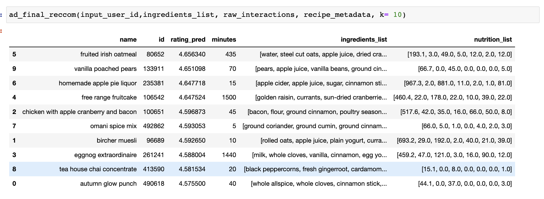
We have utilised the SVD model to generate our final recommendations. We take as input the user_id and ingredients_list (generated from output of CNN module). We constrain our recommendations with the ingredients lists, basis a threshold matching. In other words we only recommend recipes which have at least x% ingredients common with our ingredients_list. We also allow for additional filters basis protein, calories and other macros to be placed on the recommendation set.
def ad_final_reccom(user_id,ingredient_list,raw_interactions,recipe_metadata,\
                    model_file="../../models/reccomender_model1_svd.pkl",k=20,\
                    extra_filters=[],remove_old=True, threshold = 0.25):
    """
    user_id -> user ID for Recommendation Engine
    ingredient_list -> List of Ingredients from CNN Output
    raw_interactions -> The raw interactions data
    recipe_metadata -> Metadata of recipes
    threshold -> Threshold for ingredients to match
    """
    #Read Model
    model = load_pickle(model_file)
    #find recipes with similar ingredients
    mask_match_ingredients = recipe_metadata["ingredients_list"]\
        .apply(lambda x: match_ingredients(x,ingredient_list, threshold))
    #filter for extra filters
    if len(extra_filters)>0:
        combined_filter_mask = reduce(lambda x, y: x & y, extra_filters)
        mask_final = mask_match_ingredients & combined_filter_mask
    else:
        mask_final = mask_match_ingredients
    recipes_to_rank = recipe_metadata.loc[mask_final]["id"].unique()
    #remove already interacted
    if remove_old:
        # Remove already interacted items
        not_interacted, interacted = _user_items(raw_interactions, user_id)
        recipes_to_rank = list(set(recipes_to_rank)-set(interacted))
    #Score recipes
    rec_ids,rec_preds = get_reccomendation_ids(model, user_id, recipes_to_rank, k)
    df_pred = pd.DataFrame.from_dict({
        "recipe_id":rec_ids,"rating_pred":rec_preds\
        })
    meta_sub = recipe_meta_map(recipe_metadata, df_pred)
return (meta_sub[["name","id","rating_pred","minutes","ingredients_list","nutrition_list"]])- Vanilla Recomendations
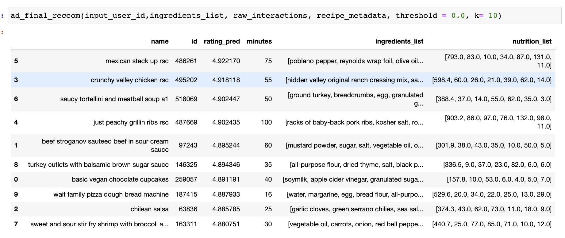
- Vanilla Recomendations + Threshold change
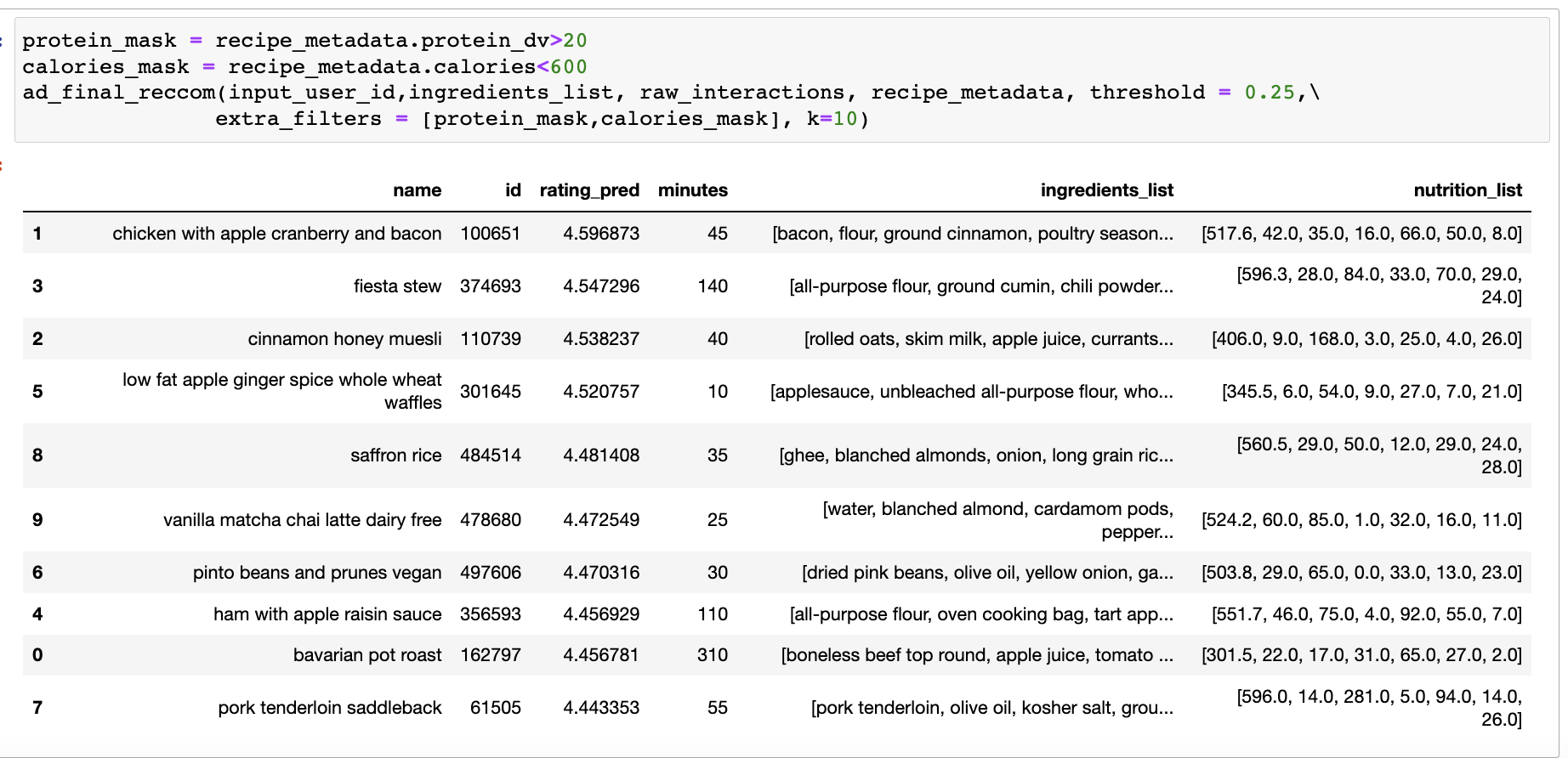
- Vanilla Recomendations + Threshold change + Macros Filter
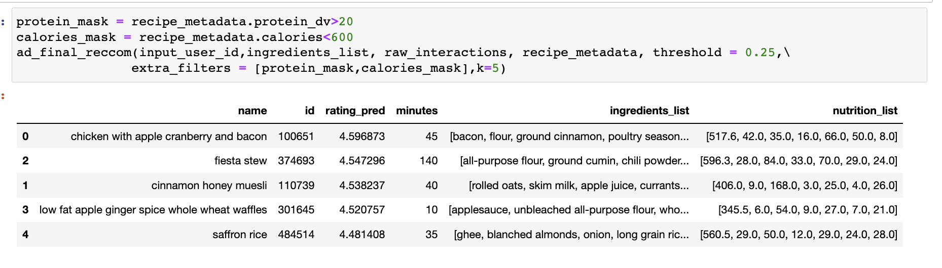
- Vanilla Recomendations + Threshold change + Macros Filter + only top 10


- Applications of NLP
- Applications of autoencoders to learn underlying feature representation and provide a more personalized recommendation.
[1]
Trang Tran, T.N., Atas, M., Felfernig, A. et al. An overview of recommender systems in the healthy food domain. J Intell Inf Syst 50, 501–526 (2018)
https://doi.org/10.1007/s10844-017-0469-0
[2]
Kaggle Data set for User food Interactions
https://www.kaggle.com/datasets/shuyangli94/food-com-recipes-and-user-interactions?select=RAW_recipes.csv
[3]
A. -S. Metwalli, W. Shen and C. Q. Wu, "Food Image Recognition Based on Densely Connected Convolutional Neural Networks," 2020 International Conference on Artificial Intelligence in Information and Communication (ICAIIC), 2020, pp. 027-032
doi: 10.1109/ICAIIC48513.2020.9065281
[4]
Food 101 DataSet
https://www.kaggle.com/datasets/dansbecker/food-101
[5] Netflix Movie Reccomedation Competition 2006 https://sifter.org/~simon/journal/20061211.html
[6] Surprise: A Python library for recommender systems, 2020 https://doi.org/10.21105/joss.02174
[7] Wide-Slice Residual Networks for Food Recognition, 2016 https://arxiv.org/pdf/1612.06543.pdf
[8] Collaborative filtering and two stage recommender system with Surprise https://www.the-odd-dataguy.com/2022/03/14/surprise/
| Sr. No. | Stage Description | Contributors |
|---|---|---|
| 1 | Classification with CNN | Manoj + Anshit + Abhinav |
| 2 | Querying Label with Ingredient Database | Yibei + Ashish + Manoj |
| 3 | Recommendation System | Abhinav + Ashish + Yibei |
| 4 | Deployment | Anshit |
Subject to alterations