Wannier90 & vASP Postprocessing module with functionalities I needed during my PhD.

Being updated Version: 0.5

1. plot_pdos

For plotting pDOS select LORBIT = 11 in INCAR file

Main function for plotting the partial density of states, for desired atoms and orbitals at all the different Wyckoff positions. Usage is straightforward:

• file = "vasprun.xml" of your VASP run, it has to contain vasprun in the name due to pymatgen handling of it.
• _atoms = Atoms whose pDOS you wanna plot as a list of strings e.g. ["P","I","O","Rn","Al"].
• _orbitals = Orbitals whose pDOS you wanna know from _atoms as a list of strings. They can be "big" orbitals (s,p,d,f) or "small" (px,py,pz,dxy,...), e.g ["s","px","d"].
• e_window = Range of energies of interest.

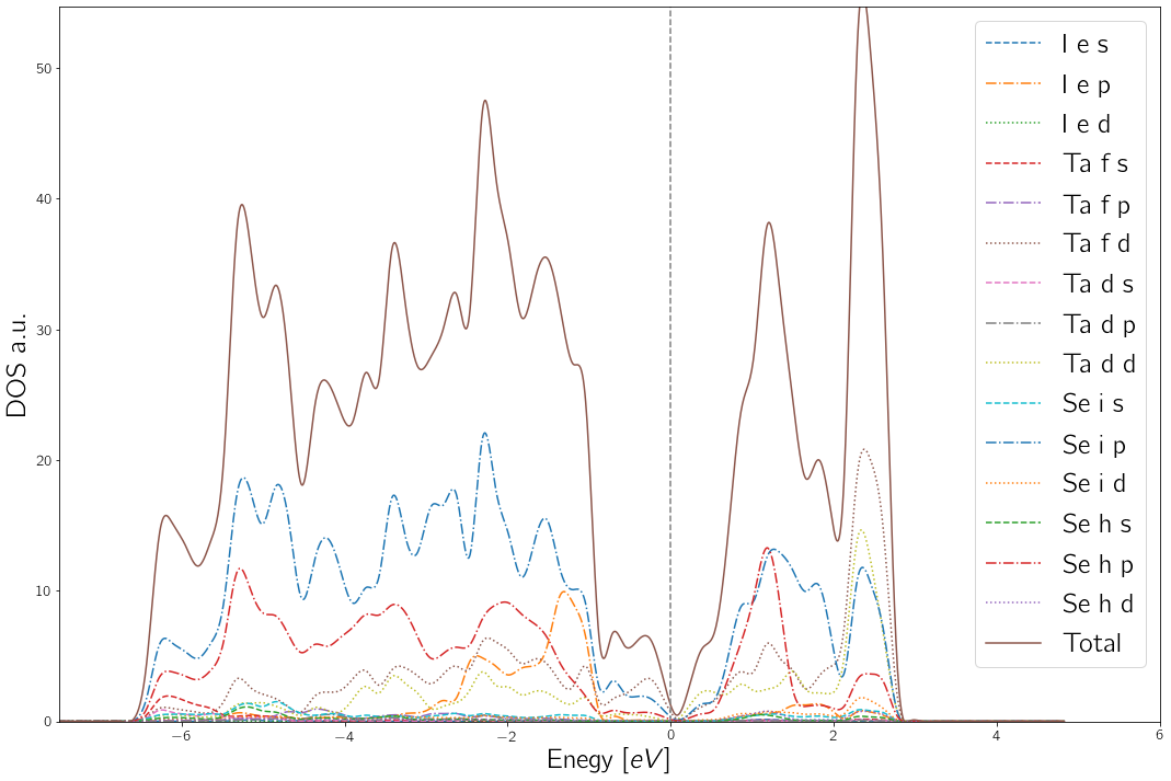
If _atoms and _orbitals are None, the function will plot every atom and big orbital at every different Wyckoff position. For a better visualization each kind of big orbital is displayed with a different linestyle.

For example (Ta6Se24I2):

wap.plot_dos("vasprun.xml",e_window = (-7.5,4))

Returns:

The first tag in the legend is the atom, the second is the Wyckoff position and the third the orbital.

2. band_counter

Counts the numebr of bands in a energy window in the whole FBZ. It gives a good clue of how to choose the energy window. Usage is as following:

wap.band_counter(file = "vasprun.xml", emin = 0.0, emax = 0.0)

• file = "vasprun.xml" of your VASP run.
• emin and emax are the lower and upper part of the energy window given in reference to Fermi energy.

For example:

wap.band_counter(file = "vasprun.xml", emin = -7.0, emax = 4.0)

Returns:

Efermi = 3.01610496.
Total bands = 544.
The number of bands between -7.00 eV (-3.98 eV) and 4.00 eV (7.02 eV) is 368.

Which is, the Fermi energy in eV, the total number of bands of the vasp run and the number of bands in the energy window (with real energies in parenthesis for wannier90.win)

3. plot_wannierbands

Function for plotting wannier bands from .dat and .gnu files.

Usage:

wap.plot_wannierbands(file_dat = "wannier90_band.dat", gnu = "wannier90_band.gnu",efermi = 0.0, e_window = None, fig_size = (15,8),savename = "wannierbands.png")

• file_dat: *_band.dat output file from a wannier90.x run.
• file_dat: *_band.gnu output file from a wannier90.x run.
• efermi: Fermi energy.
• e_window = Energy window for the plot

It generates a "wannierbands.png" file.

4 . plot_vaspbands

Function for plotting VASP bands from a non self-consistent calculation in a KPATH. Usage:

wap.plot_vaspbands(outcar = "OUTCAR", kpoints = "KPOINTS")

• outcar: OUTCAR file from VASP run.
• kpoints: KPOINTS file from nsc VASP run (linemode expected).

5. plot_comparison

Function for comparing VASP and Wannier90 bandstructures combining the previous functions and tags. Usage:

wap.plot_comparison(outcar = "OUTCAR", kpoints = "KPOINTS",file_dat = "wannier90_band.dat", gnu = "wannier90_band.gnu",efermi = 0.0, fig_size = (12,8), e_window = (-4,4),savename = "comparison.png"):

• outcar: OUTCAR file from VASP run.
• kpoints: KPOINTS file from nsc VASP run (linemode expected).
• file_dat: *_band.dat output file from a wannier90.x run.
• file_dat: *_band.gnu output file from a wannier90.x run.
• efermi: Fermi energy.
• e_window = Energy window for the plot

Example: RhSi

wap.plot_comparison(outcar = "OUTCAR", kpoints = "KPOINTS",file_dat = "wannier90_band.dat", gnu = "plottt/wannier90_band.gnu",efermi = 0.0, fig_size = (12,8), e_window = (-4,4),savename = "comparison.png") 

6. wann_kpoints

Function for generating kpath string for seedname.win using a KPOINT file from a nsc VASP calculation. Usage is as follows:

wann_kpoints(file = "KPOINTS")

Where KPOINTS is like:

Cubic
20   ! 20 grids
Line-mode
reciprocal
   0.000   0.000   0.000   ! GAMMA
   0.000   0.500   0.000   ! X
   0.000   0.500   0.000   ! X
   0.500   0.500   0.000   ! M
   0.500   0.500   0.000   ! M
   0.000   0.000   0.000   ! GAMMA
   0.000   0.000   0.000   ! GAMMA
   0.500   0.500   0.500   ! R
   0.500   0.500   0.500   ! R
   0.000   0.500   0.000   ! X
   0.500   0.500   0.000   ! M
   0.500   0.500   0.500   ! R

And it generates a WKPTS.txt file as:

G 0.000 0.000 0.000 X 0.000 0.500 0.000 
X 0.000 0.500 0.000 M 0.500 0.500 0.000 
M 0.500 0.500 0.000 G 0.000 0.000 0.000 
G 0.000 0.000 0.000 R 0.500 0.500 0.500 
R 0.500 0.500 0.500 X 0.000 0.500 0.000 
M 0.500 0.500 0.000 R 0.500 0.500 0.500 

7. plot_custom_vaspbands

Similar to plot_vaspbands but more customizable. Usage is as follows:

wap.plot_custom_vaspbands(outcar = "OUTCAR",kpoints = "KPOINTS",
                          figsize = (10,7.5),ewindow = (-3,3),
                          dpi = 500,linewidth = 0.5,
                          kp_i=None,kp_f=None,
                          title=None,fname=None)

Where:

• kp_i & kp_f is the number of the fist and last KPOINT in the path that you want to plot. E.g. in the KPOINTS file from above example kp_i = 2 would correspond to M.
• title and fname are the title to be printed in the figure and the path to the figure when saved.

8. tb_to_hr Generate a seedname_hr.dat from seedname_tb.dat. Usage is as follows:

wap.tb_to_hr(file = "wannier90_tb.dat")

compare_MBJ

Function for comparing PBE nscc and MBJ scc functional bandstructures using pymatgen treatment of vasprun.

wap.compare_MBJ(vasprun_pbe = "vasprun1.xml",
            vasprun_mbj = "vasprun2.xml",
            kpoint_file = "KPOINTS",
            e_window = (-4,4),
            fig_title = None,
            fig_name = "comparison.png")

Usage:

• vasprun_pbe: vasprun file for PBE nsc run.
• vasprun_mbj: vasprun file for MBJ scc run.
• kpoint_file: kpoint file for nsc (linemode expected).

For example:

wap.compare(vasprun_pbe = "vasprun81_rel.xml",
            vasprun_mbj = "vasprun81.xml",
            kpoint_file = "KPOINTS",
            e_window = (-2,2),
            fig_title = "SG81",
            fig_name = "comparison81.png")

Returns:

More functionalities are present in the code and many more are coming, stay tuned & take a look at WASPP05.py. （＾³＾）～♪

Package Requeriments:

• numpy
• matplotlib
• scipy
• itertools
• re
• pymatgen

This code is heavily based in the one by Martín Gutierrez @mgamigo for QEspresso, PyBand by Qijing Zheng & Chengcheng Xiao and uses pymatgen.