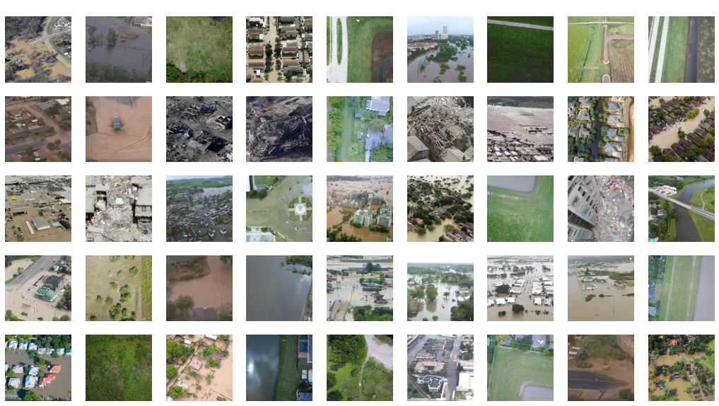
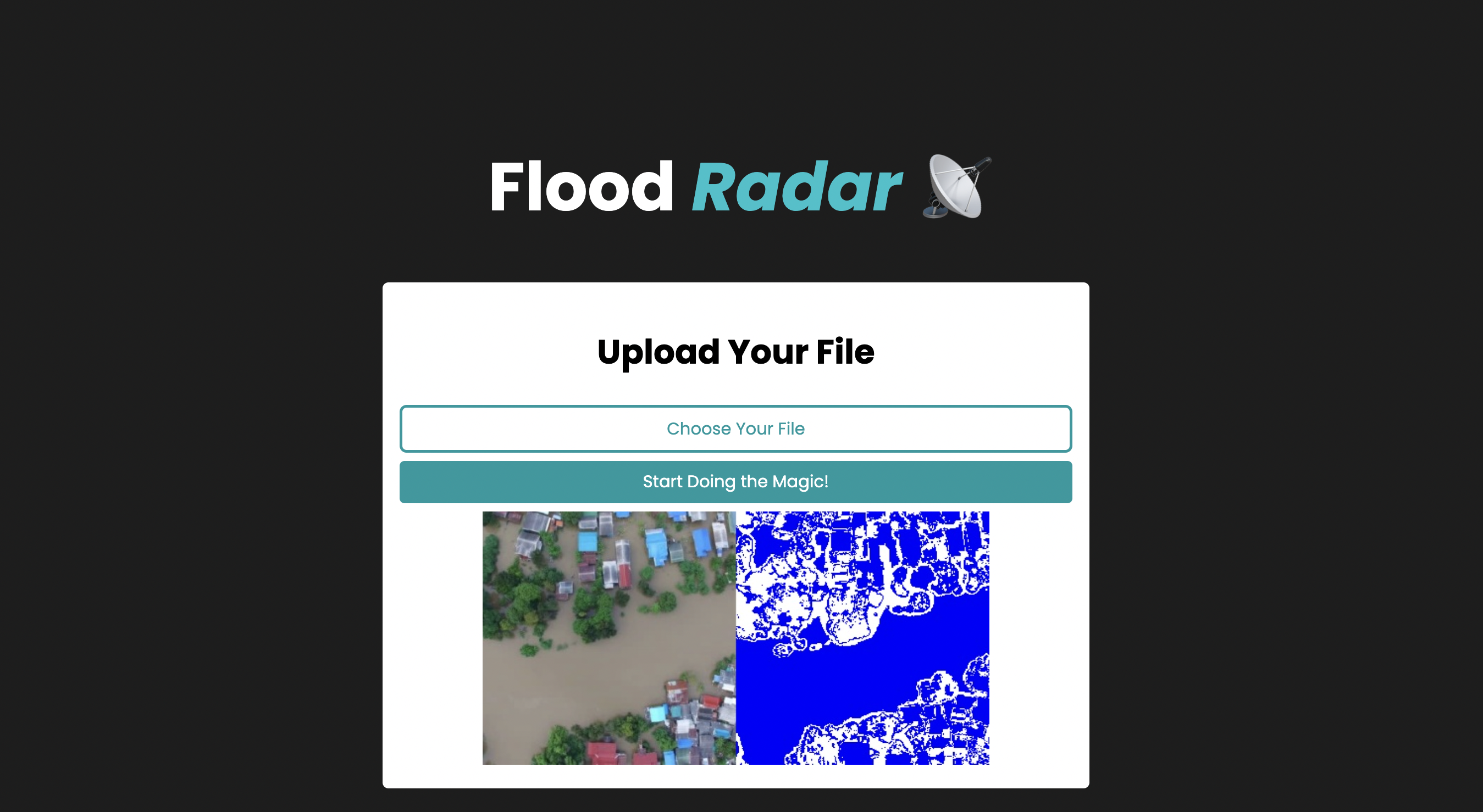
The aim of this project is to utilize computer vision for the purpose of detecting images involving a flood and localizing the flooded areas within them in an automated fashion using classical machine learning and computer vision techniques. Such system shall be useful if employed on a satellite to provide critical information to emergency response teams such as the areas and degrees of flood.
We solved the detection problem by employing the following pipeline

The following is the implied folder structure:
.
├── DataPreparation
│   ├── DataPreparation.ipynb
│   └── DataPreparation.py
├── FeatureExtraction
│   ├── Glcm
│   │   ├── Glcm.ipynb
│   │   └── Glcm.py
│   ├── Hist
│   │   ├── Hist.ipynb
│   │   └── Hist.py
│   ├── Resnet
│   │   ├── Resnet.ipynb
│   │   └── Resnet.py
│   ├── Shufflenet
│   │   ├── Shufflenet.ipynb
│   │   └── Shufflenet.py
│   └── Visuals.py
├── ModelPipelines
│   ├── CNN
│   │   └── CNN.ipynb
│   ├── ISODATA
│   │   ├── ISODATA.ipynb
│   │   └── ISODATA.py
│   ├── KMeans
│   │   ├── KMeans.ipynb
│   │   ├── KMeans.py
│   │   └── water.jpg
│   ├── LogisticRegression
│   │   ├── HOG-LogisticRegression.ipynb
│   │   └── LBP-LogisticRegression.ipynb
│   ├── QDA
│   │   ├── Hist-QDA.ipynb
│   │   └── LBP-QDA.ipynb
│   ├── SVM
│   │   ├── Deep-SVM.ipynb
│   │   ├── Glcm-SVM.ipynb
│   │   ├── HOG-SVM.ipynb
│   │   ├── Hist-SVM.ipynb
│   │   ├── LBP-SVM.ipynb
│   │   └── Shuffle-SVM.ipynb
│   └── SimpleFeatures
│       └── SimpleFeatures.py
├── Production
│   └── Flask
├── Quests
├── README.md
├── References
│   ├── Flood-Paper.pdf
│   ├── Relatively Meh Paper.pdf
│   └── SI Project.pdf
├── requirements.txt
└── script.ipynb
pip install requirements.txt
# To run any stage of the pipeline, consider the stage's folder. There will always be a demonstration notebook.
The project is also fully equipped to run on Google collab if the project's folder is synchronized with your Google drive. You may reach out to any of the developers if you find any difficulty in running it there.
We have set the following set of working standards as we were undertaking the project. If you wish to contribute for any reason then please respect such standards.
We shall illustrate the pipeline in the rest of the README. For an extensive overview of the project you may choose also checking the report and the slides or the demonstration notebooks herein.
The given dataset involves 922 images equally divided into flooded and non-flooded images that vary significantly in terms of the quality, size and content. We employed a data processing stage with the following capabilities:
- Reading the images
- Image Standardization
- Greyscale Conversion
- Center-cropping with Maximal Content
- Swapping Channels
- Tensor Conversions and Custom Processing
- Saving the preprocessed images
We have considered the following set of features
| GLCM | ColorHistogram | Histogram of Gradients | Local Binary Pattern | ResNet | ShuffleNet |
|---|
where in all cases PCA was also an option.
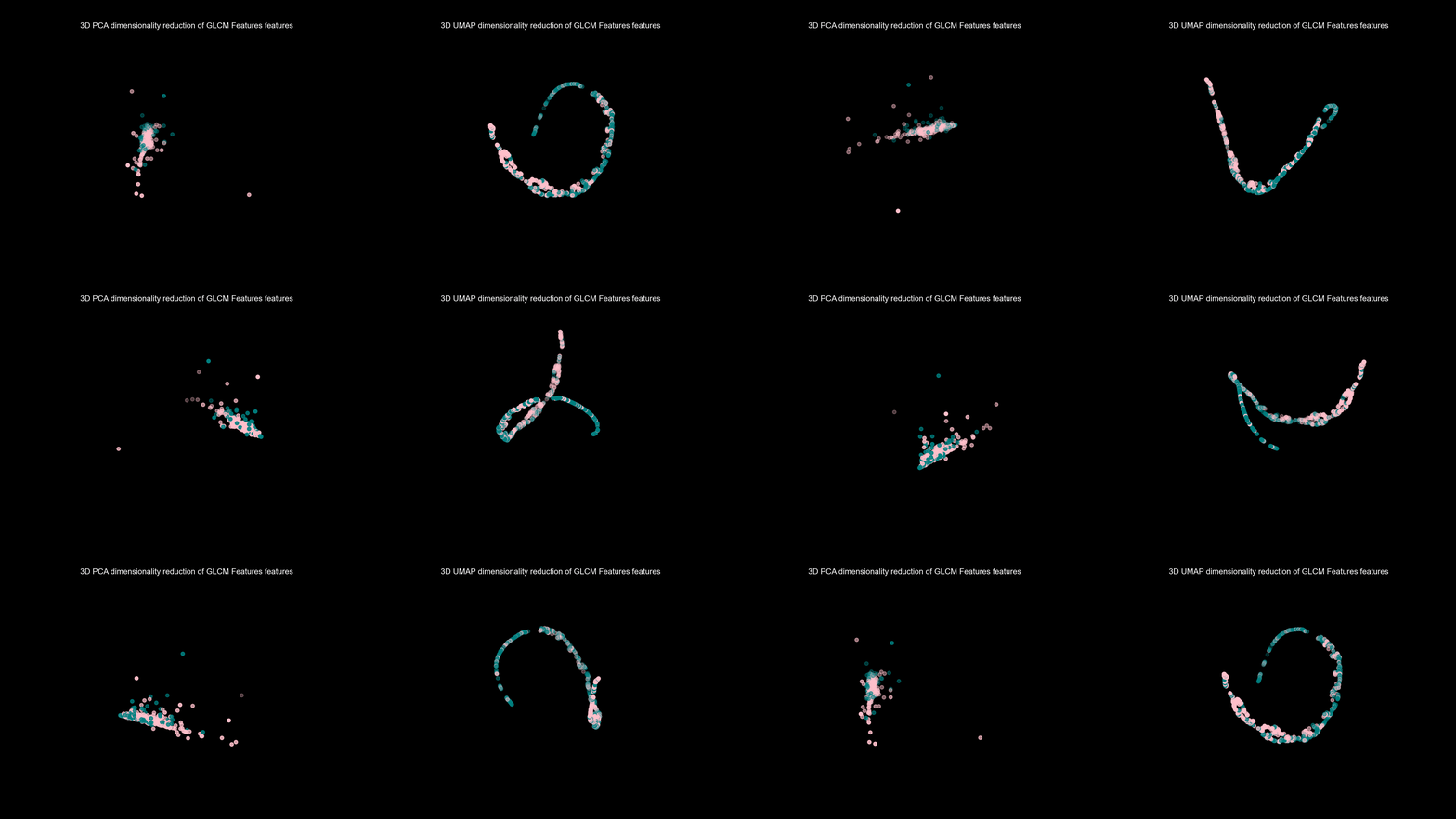
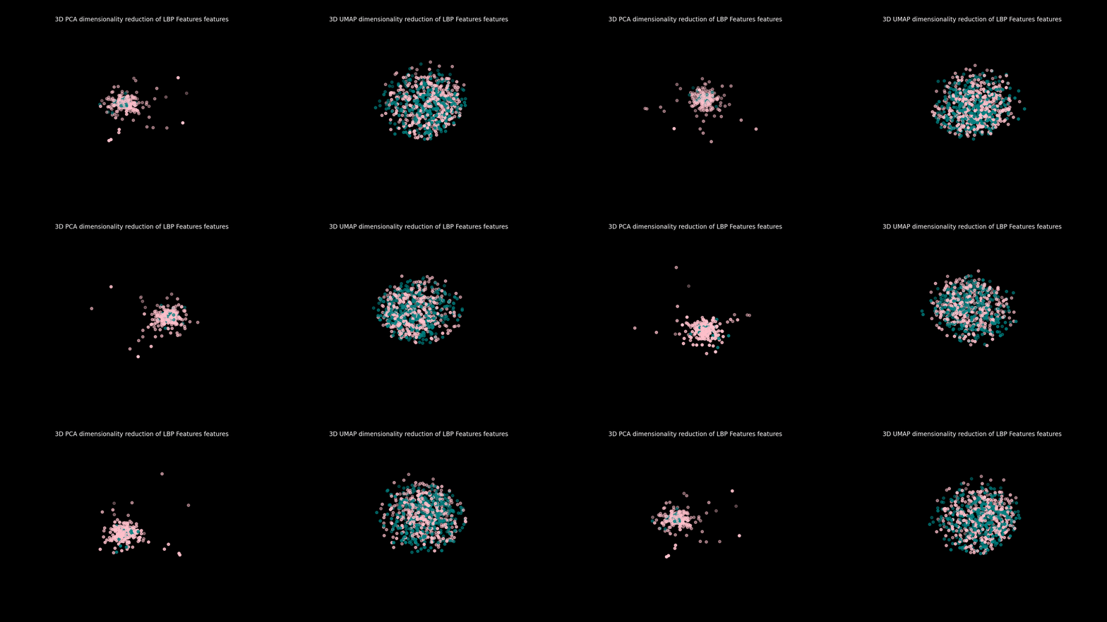
GLCM features are just statistics acquired from the gray-level co-occurrence matrix of the image. The following analyzes the target's separability under all possible pairs of GLCM features
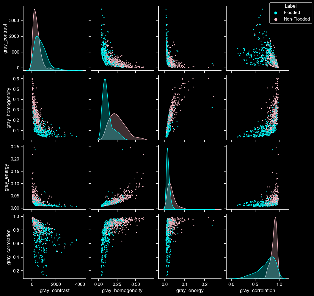
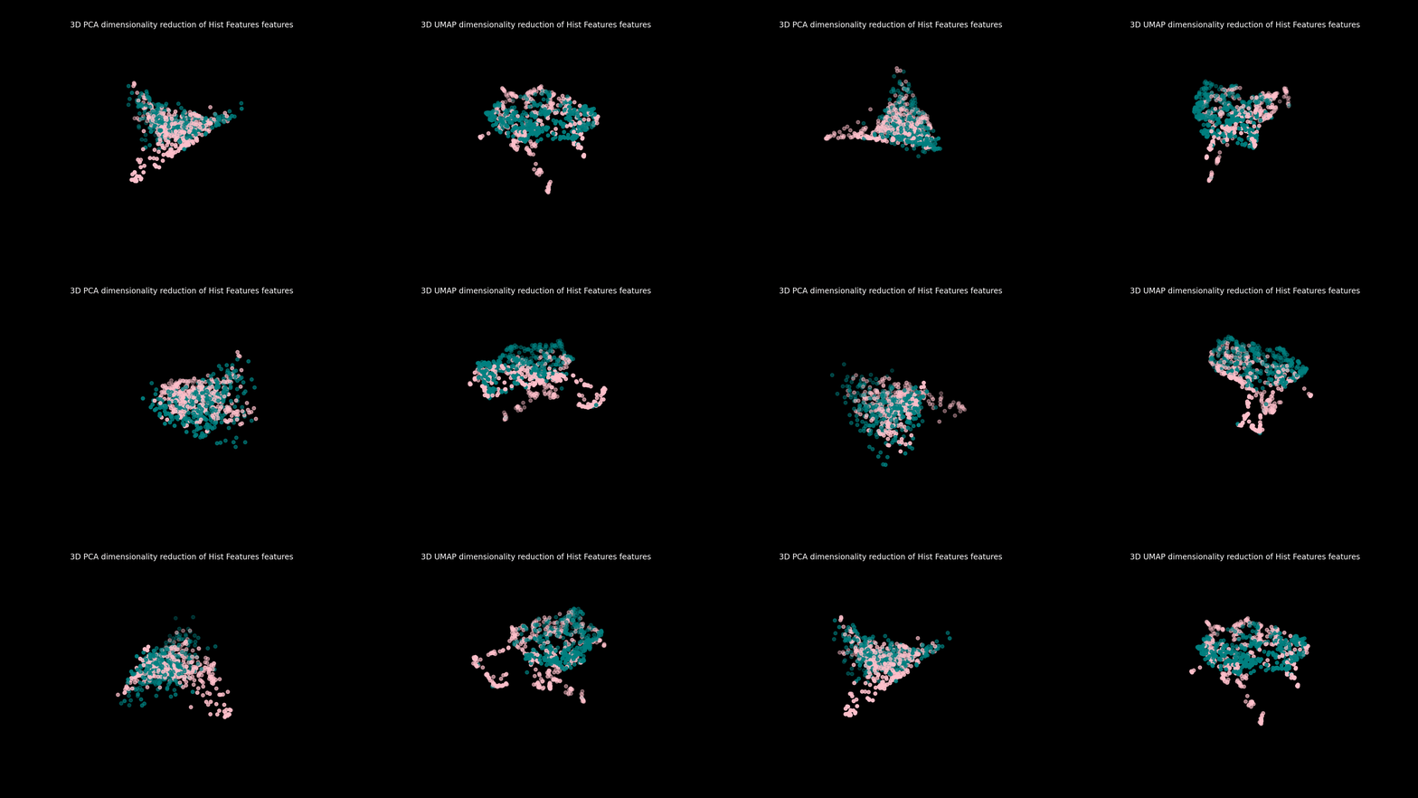
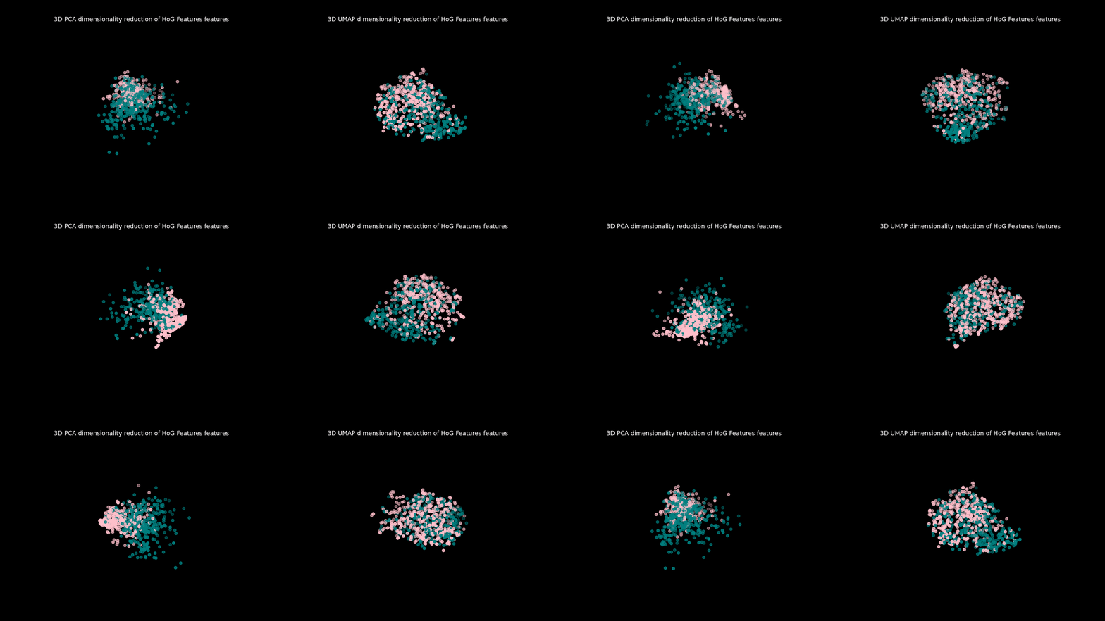
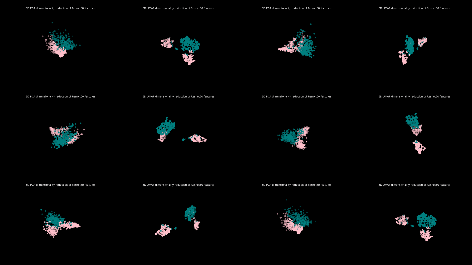
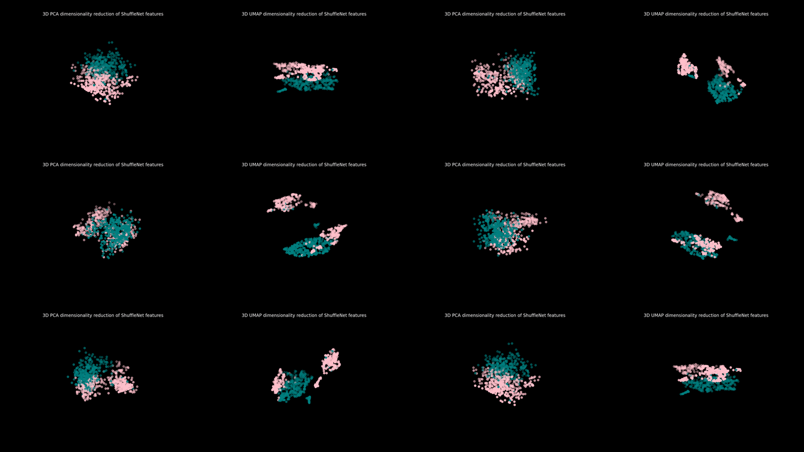
To illustrate all of them together, we have utilized linear (PCA) and non-linear (UMAP) dimensioanlity reduction
In this, we simply sampled the color histogram to form a feature vector for the image. Surprisingly better than expected.
In this, we simply described the image by a histogram of gradients; this is useful since edges carry important info about whether the image contains a flood or not.
A sliding window over the image is used to detect patterns between the center pixel and the rest of the pixels; hence, detecting repeating patterns. This is helpful since flooded images will often lack texture compared to non-flooded ones.
Eventually, we decided to try features extracted by deep learning computer vision models. Our first choice was the ResNet-50 CNN model.
Notice that it is no longer fruit salad.
After a thorough comparison of various transfer learning options, we found it opportune to try out ShuffleNet features - a light-weight model with performance that matches or exceeds much larger models such as ResNet-50.
| Model | Features | |||||
|---|---|---|---|---|---|---|
| CNN | Raw Images | |||||
| Logistic Regression | Hog | LBP | ||||
| Bayes Classifier | ColorHist | LBP | ||||
| SVM | ResNet | GLCM | ColorHist | HoG | LBP | ShuffleNet |
We built a CNN using Pytorch Lightning, converging with LeNet after a lot of hyperparameter tuning. Performance was not overly spectacular.
For the rest of the pipelines, we used extracted features as shown above. We also used in-notebook logging using the MLPath library as present in the demonstration notebooks and the report. The following shows a sample of the log for the LBP-Logistic pipeline:
| info | read_data | get_lbp | apply_pca | LogisticRegression | metrics | |||||||||||||||||||
|---|---|---|---|---|---|---|---|---|---|---|---|---|---|---|---|---|---|---|---|---|---|---|---|---|
| time | date | duration | id | gray | saved | new_size | normalize | transpose | radius | n_components | pca_obj | penalty | C | dual | tol | fit_intercept | intercept_scaling | solver | max_iter | multi_class | verbose | warm_start | Accuracy | F1 |
| 14:29:58 | 05/20/23 | 1.10 min | 1 | True | True | 256 | False | False | 5 | 512 | PCA(n_components=512) | l2 | 7 | False | 0.0 | True | 1 | lbfgs | 100 | auto | 0 | False | 0.5891891891891892 | 0.5313333333333333 |
| 14:31:55 | 05/20/23 | 34.83 s | 2 | True | True | 256 | False | False | 5 | l2 | 7 | False | 0.0 | True | 1 | lbfgs | 100 | auto | 0 | False | 0.5837837837837838 | 0.5633716475095785 | ||
| 14:38:15 | 05/20/23 | 1.73 min | 8 | True | True | 256 | False | False | 4 | 512 | PCA(n_components=512) | l2 | 100 | False | 0.0 | True | 1 | lbfgs | 100 | auto | 0 | False | 0.7567567567567568 | 0.756043956043956 |
Note that hyperparameter search was also used for high-performing models such as SVM.
For evaluation, we used a 20% validation set split and 10-Repeated-5-Fold Cross Validation for more fine-grained comparisons (e.g., ShuffleNet VS. ResNet). The following portrays the results:
| Method | HOG-LR | LBP-LR | GLCM-SVM | HOG-SVM | LBP-SVM | Shufflenet-SVM | Resnet-SVM | Hist-QDA | LBP-QDA |
|---|---|---|---|---|---|---|---|---|---|
| F1-score | 0.854 | 0.756 | 0.683 | 0.897 | 0.832 | 0.989 | 0.979 | 0.816 | 0.619 |
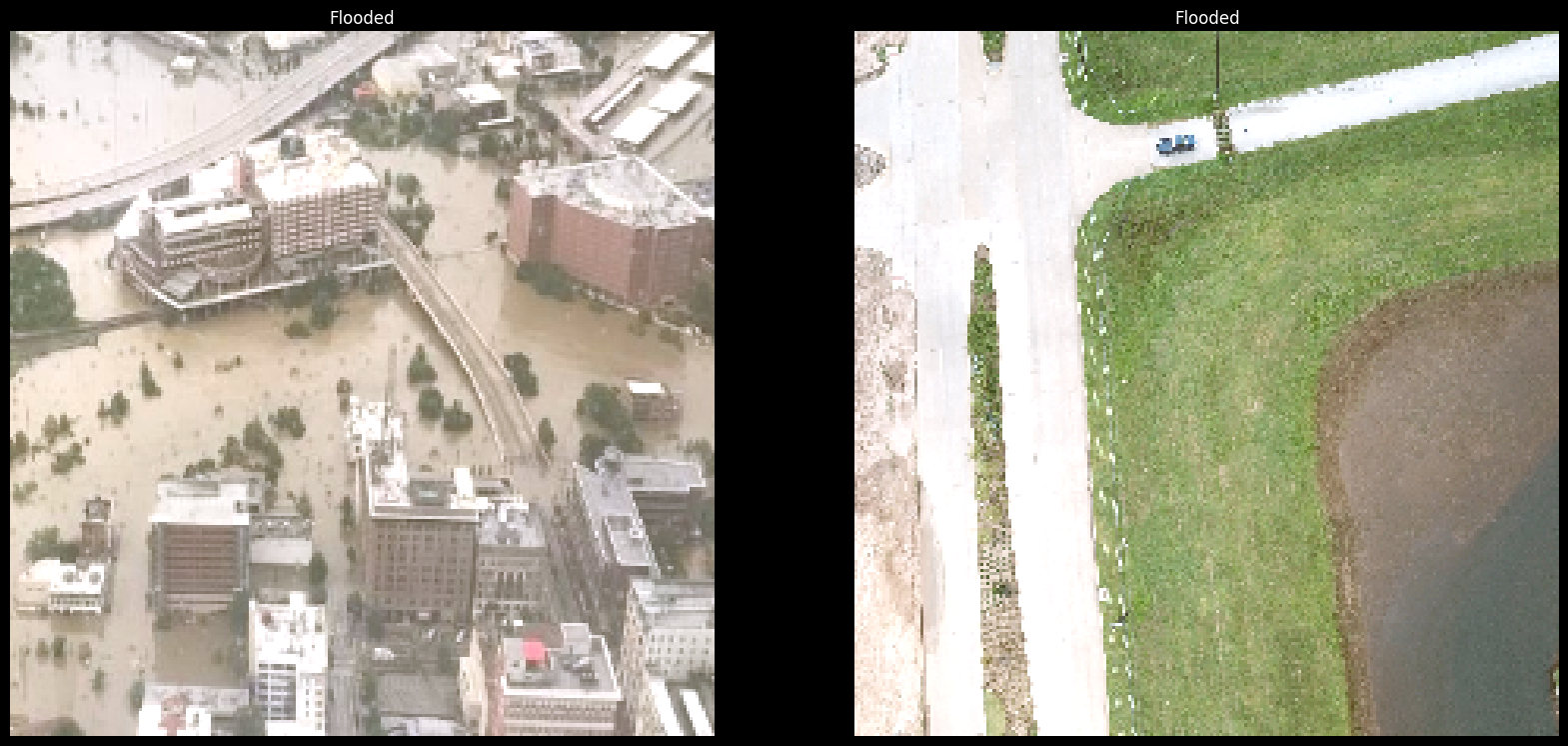
Overall, ShuffleNet was our best model. In light of manual error analysis, there were its mistakes on the validation set
After submitting ShuffleNet to the competition, we found that it has ranked only 4th place relative to the other accuracies in the leaderboard with an accuracy of 96.5%. We requested the test set to do some retrospective analysis and found out that ResNet actually performs significantly better on the test set at 98% (contrary to performance on the original dataset where ShuffleNet had 98% and ResNet had 97.7% under 10-repeated-5-Fold cross validation) and that ShuffleNet has made mistakes for the following
After revisiting 10-Repeated-5-Fold cross validation for both ResNet and ShuffleNet we concluded that over the 50 random validation splits, the standard deviation was as large as 1.1% for ResNet and 1% for ShuffleNet which is even further aggravated for 10-Repeated-10-Fold cross validation. We could only explain this unexpectedly high sensitivity to the split by the large variance inherent in the data itself as it seems to be collected from different sources. This signals that decisions taken by individuals under a fixed validation set may be really sensitive on how it tallies with the actual test set which is randomly decided; the STD is high compared to a typical dataset.
For this task, we considered ISODATA and K-Means to segment the flooded images. K-Means proved more successful on that front.
Two obstacles in this task were red water and luminance effects our approach to circumventing them involved swapping channels and utiliting HSV channels respectivelty.
Classic Example
Red Water
Luminance Problems
Such masterpiece surely deserved a
cd Production/Flask
flask run|
Essam |
MUHAMMAD SAAD |
Noran Hany |
Halahamdy22 |
We have utilized Notion for progress tracking and task assignment among the team.
