A graph is a data structure that represents a collection of interconnected nodes through a set of edges.

This abstract structure is highly versatile and finds applications in various domains, from social network analysis to computer networking.

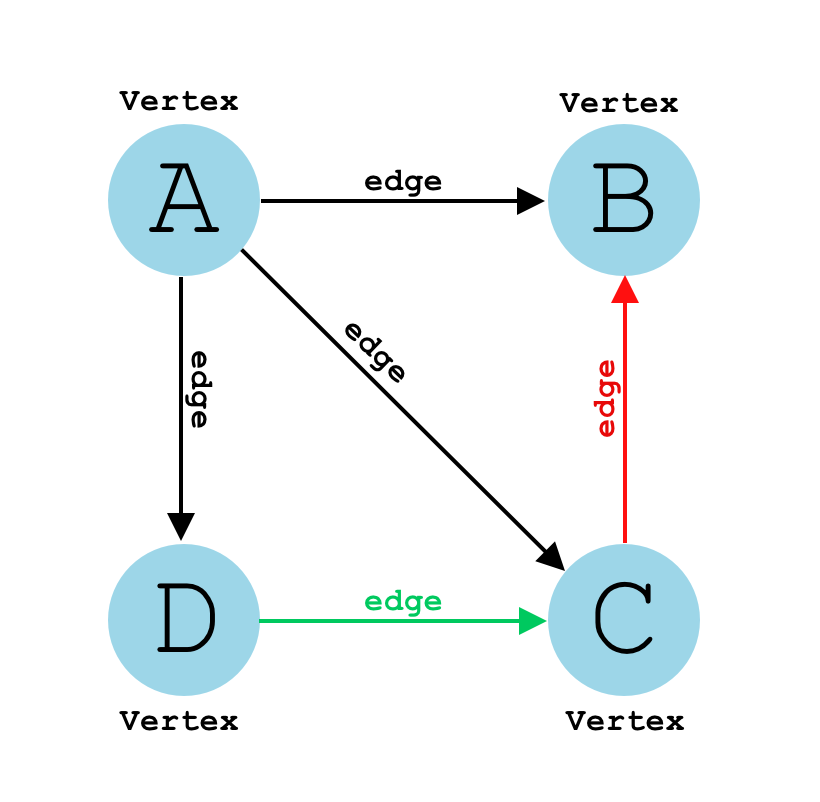
A graph consists of two main components:

1. Nodes: Also called vertices, these are the fundamental units that hold data.
2. Edges: These are the connections between nodes, and they can be either directed or undirected.

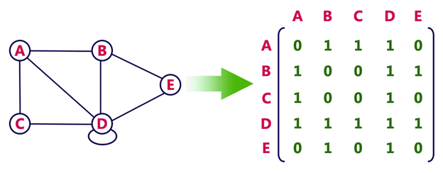
There are several ways to represent graphs in computer memory, with the most common ones being adjacency matrix, adjacency list, and edge list.

In an adjacency matrix, a 2D Boolean array indicates the edges between nodes. A value of True at index [i][j] means that an edge exists between nodes i and j.

Here is the Python code:

graph = [
    [False, True, True],
    [True, False, True],
    [True, True, False]
]

An adjacency list represents each node as a list, and the indices of the list are the nodes. Each node's list contains the nodes that it is directly connected to.

Here is the Python code:

graph = {
    0: [1, 2],
    1: [0, 2],
    2: [0, 1]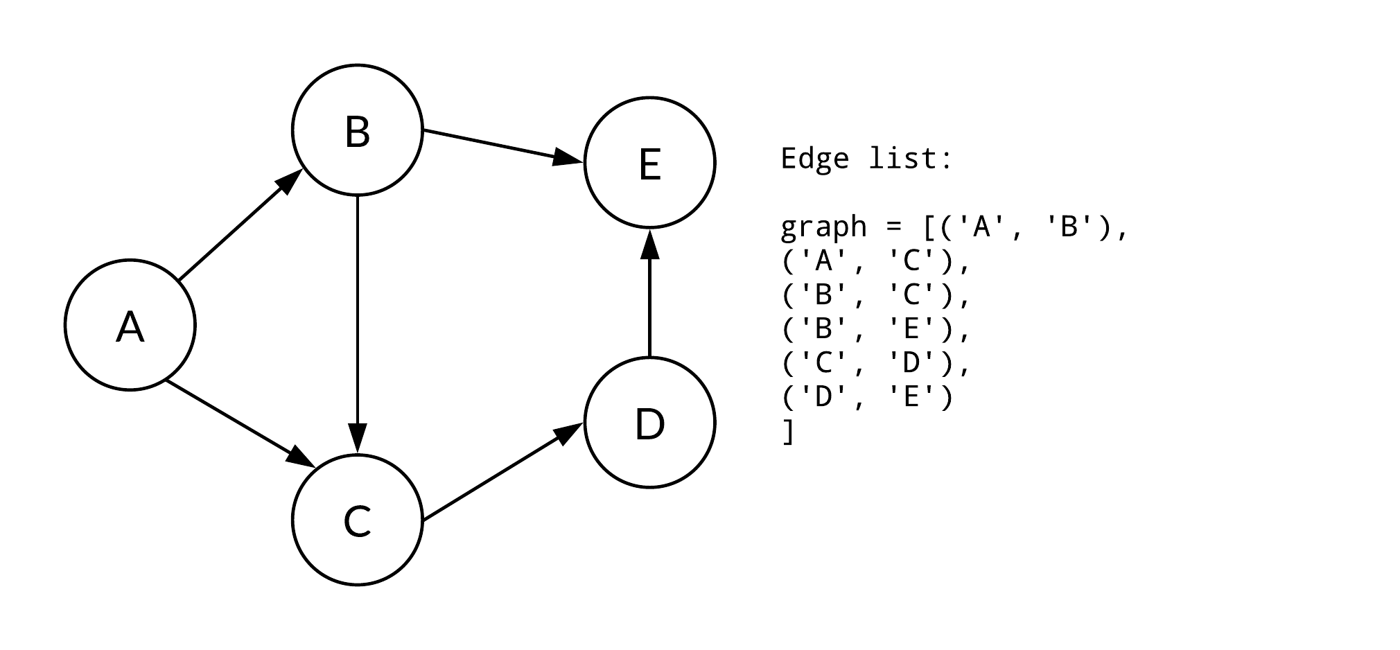
}

An edge list is a simple list of tuples, where each tuple represents an edge between two nodes.

Here is the Python code:

graph = [(0, 1), (0, 2), (1, 2)]

Graphs serve as adaptable data structures for various computational tasks and real-world applications. Let's look at their diverse types.

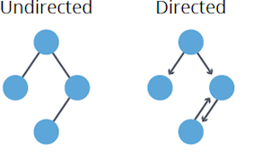
1. Undirected: Edges lack direction, allowing free traversal between connected nodes. Mathematically, $(u,v)$ as an edge implies $(v,u)$ as well.
2. Directed (Digraph): Edges have a set direction, restricting traversal accordingly. An edge $(u,v)$ doesn't guarantee $(v,u)$.

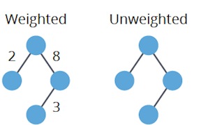
1. Weighted: Each edge has a numerical "weight" or "cost."
2. Unweighted: All edges are equal in weight, typically considered as 1.

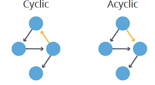
1. Cyclic: Contains at least one cycle or closed path.
2. Acyclic: Lacks cycles entirely.

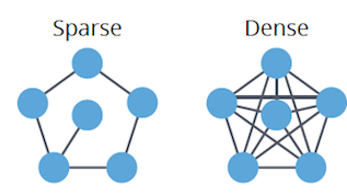
1. Dense: High edge-to-vertex ratio, nearing the maximum possible connections.
2. Sparse: Low edge-to-vertex ratio, closer to the minimum.

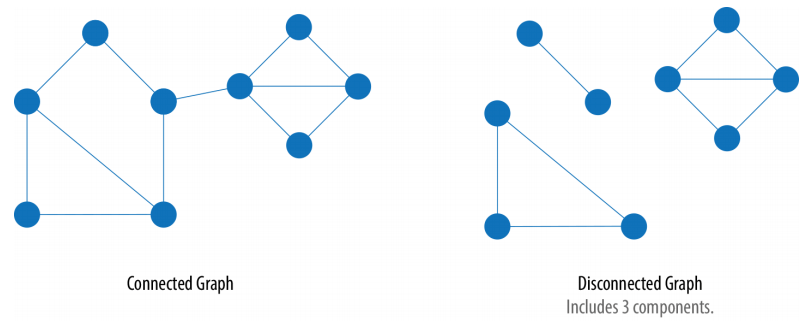
1. Connected: Every vertex is reachable from any other vertex.
2. Disconnected: Some vertices are unreachable from others.

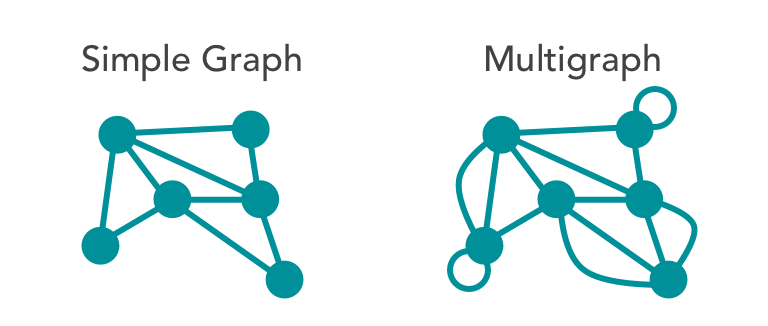
1. Multigraph: Allows duplicate edges between vertices.
2. Simple: Limits vertices to a single connecting edge.

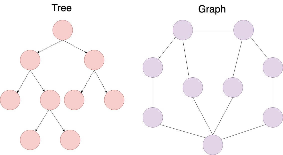
Graphs and trees are both nonlinear data structures, but there are fundamental distinctions between them.

• Uniqueness: Trees have a single root, while graphs may not have such a concept.
• Topology: Trees are hierarchical, while graphs can exhibit various structures.
• Focus: Graphs center on relationships between individual nodes, whereas trees emphasize the relationship between nodes and a common root.

• Elements: Composed of vertices/nodes (denoted as V) and edges (E) representing relationships. Multiple edges and loops are possible.
• Directionality: Edges can be directed or undirected.
• Connectivity: May be disconnected, with sets of vertices that aren't reachable from others.
• Loops: Can contain cycles.

• Elements: Consist of nodes with parent-child relationships.
• Directionality: Edges are strictly parent-to-child.
• Connectivity: Every node is accessible from the unique root node.
• Loops: Cycles are not allowed.

To ensure a graph remains connected, it must have a minimum number of edges determined by the number of vertices. This is known as the edge connectivity of the graph.

The minimum number of edges required for a graph to remain connected is given by:

$$ \text{{Edge Connectivity}} = \max(\delta(G),1) $$

Where:

• $\delta(G)$ is the minimum degree of a vertex in $G$.
• The maximum function ensures that the graph remains connected even if all vertices have a degree of 1 or 0.

For example, a graph with a minimum vertex degree of 3 or more requires at least 3 edges to stay connected.

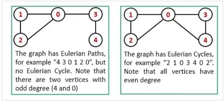
In graph theory, an Euler Path and an Euler Circuit serve as methods to visit all edges (links) exactly once, with the distinction that an Euler Circuit also visits all vertices once.

A graph has an Euler Path if it contains exactly two vertices of odd degree.

A graph has an Euler Circuit if every vertex has even degree.

Degree specifies the number of edges adjacent to a vertex.

• Starting Vertex: In an Euler Path, the unique starting and ending vertices are the two with odd degrees.
• Reachability: In both Euler Path and Circuit, every edge must be reachable from the starting vertex.
• Direction-Consistency: While an Euler Path is directionally open-ended, an Euler Circuit is directionally closed.

Graphs can be represented in various ways, but Adjacency Matrix and Adjacency List are the most commonly used data structures. Each method offers distinct advantages and trade-offs, which we'll explore below.

• Adjacency Matrix: Requires a $N \times N$ matrix, resulting in $O(N^2)$ space complexity.
• Adjacency List: Utilizes a list or array for each node's neighbors, leading to $O(N + E)$ space complexity, where $E$ is the number of edges.

• Adjacency Matrix: Constant time, $O(1)$, as the presence of an edge is directly accessible.
• Adjacency List: Up to $O(k)$, where $k$ is the degree of the vertex, as the list of neighbors may need to be traversed.

• Adjacency Matrix: Requires $O(N^2)$ time to iterate through all potential edges.
• Adjacency List: Takes $O(N + E)$ time, often faster for sparse graphs.

• Adjacency Matrix: $O(1)$ for both addition and removal, as it involves updating a single cell.
• Adjacency List: $O(k)$ for addition or removal, where $k$ is the degree of the vertex involved.

• Adjacency Matrix: $O(N^2)$ as resizing the matrix is needed.
• Adjacency List: $O(1)$ as it involves updating a list or array.

Here is the Python code:

adj_matrix = [
    [0, 1, 1, 0, 0, 0],
    [1, 0, 0, 1, 0, 0],
    [1, 0, 0, 0, 0, 1],
    [0, 1, 0, 0, 1, 1],
    [0, 0, 0, 1, 0, 0],
    [0, 0, 1, 1, 0, 0]
]

adj_list = [
    [1, 2],
    [0, 3],
    [0, 5],
    [1, 4, 5],
    [3],
    [2, 3]
]

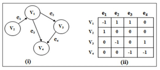
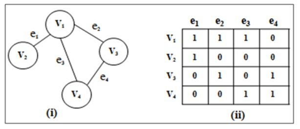
An incidence matrix is a binary graph representation that maps vertices to edges. It's especially useful for directed and multigraphs. The matrix contains $0$s and $1$s, with positions corresponding to "vertex connected to edge" relationships.

• Columns: Represent edges
• Rows: Represent vertices
• Cells: Indicate whether a vertex is connected to an edge

Each unique row-edge pair depicts an incidence of a vertex in an edge, relating to the graph's structure differently based on the graph type.

• Algorithm Efficiency: Certain matrix operations can be faster than graph traversals.
• Graph Comparisons: It enables direct graph-to-matrix or matrix-to-matrix comparisons.
• Database Storage: A way to represent graphs in databases amongst others.
• Graph Transformations: Useful in transformations like line graphs and dual graphs.

Edge list is a straightforward way to represent graphs. It's apt for dense graphs and offers a quick way to query edge information.

• Edge Storage: The list contains tuples (a, b) to denote an edge between nodes $a$ and $b$.
• Edge Direction: The edges can be directed or undirected.
• Edge Duplicates: Multiple occurrences signal multigraph. Absence ensures simple graph.

Here is the Python 3 code:

# Example graph
edges = {('A', 'B'), ('A', 'C'), ('B', 'C'), ('C', 'D'), ('B', 'D'), ('D', 'E')}

# Check existence
print(('A', 'B') in edges)  # True
print(('B', 'A') in edges)  # False
print(('A', 'E') in edges)  # False

# Adding an edge
edges.add(('E', 'C'))

# Removing an edge
edges.remove(('D', 'E'))

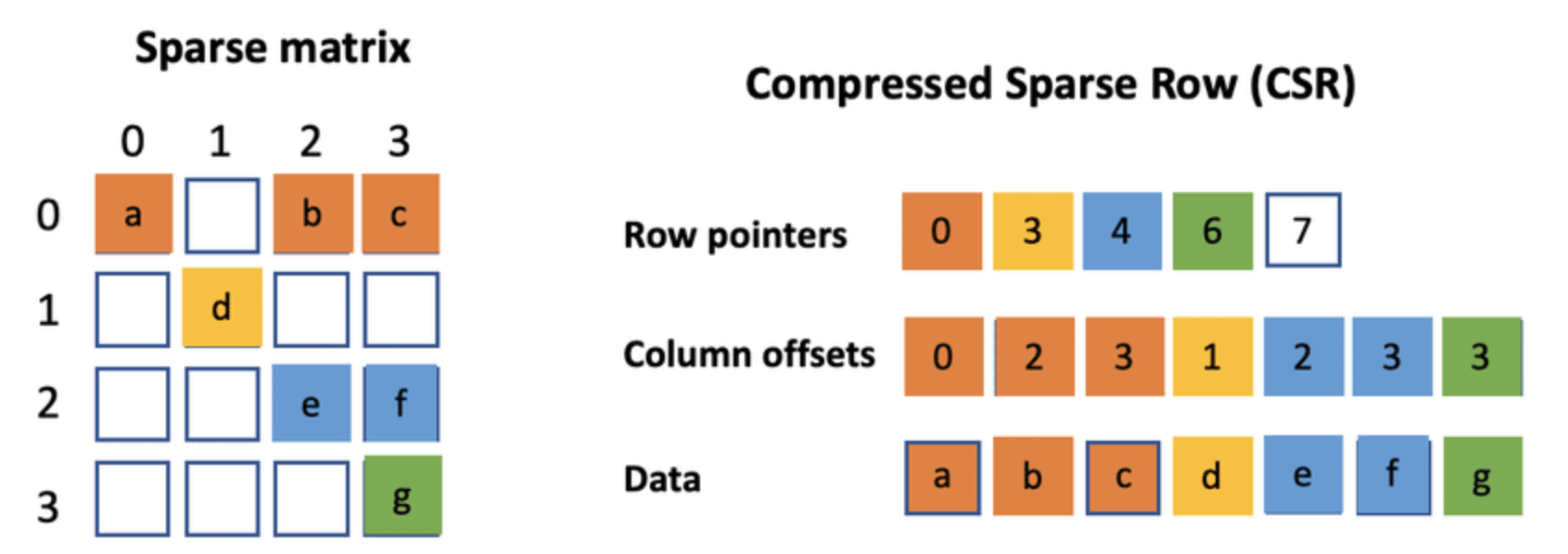
print(edges)  # Updated set: {('A', 'C'), ('B', 'D'), ('C', 'D'), ('A', 'B'), ('E', 'C'), ('B', 'C')}

In Compressed Sparse Row format, the graph is represented by three linked arrays. This streamlined approach can significantly reduce memory use and is especially beneficial for sparse graphs.

Let's go through the data structures and the detailed process.

1. Indptr Array (IA): A list of indices where each row starts in the adj_indices array. It's of length n_vertices + 1.
2. Adjacency Index Array (AA): The column indices for each edge based on their position in the indptr array.
3. Edge Data: The actual edge data. This array's length matches the number of non-zero elements.

Here is the Python code:

indptr = [0, 2, 3, 5, 6, 7, 8]
indices = [2, 4, 0, 1, 3, 4, 2, 3]
data = [1, 2, 3, 4, 5, 6, 7, 8]

# Reading from the CSR Format
for i in range(len(indptr) - 1):
    start = indptr[i]
    end = indptr[i + 1]
    print(f"Vertex {i} is connected to vertices {indices[start:end]} with data {data[start:end]}")

# Writing a CSR Represented Graph
# Vertices 0 to 5, Inclusive.
# 0 -> [2, 3, 4] - Data [3, 5, 7]
# 1 -> [0] - Data [1]
# 2 -> [] - No outgoing edges.
# 3 -> [1] - Data [2]
# 4 -> [3] - Data [4]
# 5 -> [2] - Data [6]

# Code to populate:
# indptr =  [0, 3, 4, 4, 5, 6, 7]
# indices = [2, 3, 4, 0, 1, 3, 2]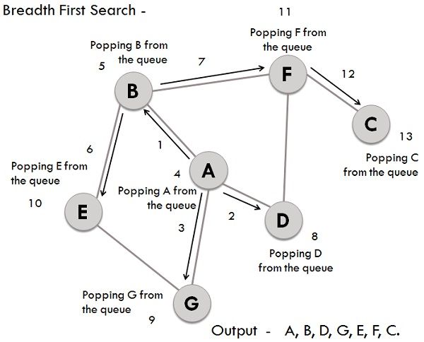
# data = [3, 5, 7, 1, 2, 4, 6]

Breadth-First Search (BFS) is a graph traversal technique that systematically explores a graph level by level. It uses a queue to keep track of nodes to visit next and a list to record visited nodes, avoiding redundancy.

• Queue: Maintains nodes in line for exploration.
• Visited List: Records nodes that have already been explored.

1. Initialize: Choose a starting node, mark it as visited, and enqueue it.
2. Explore: Keep iterating as long as the queue is not empty. In each iteration, dequeue a node, visit it, and enqueue its unexplored neighbors.
3. Terminate: Stop when the queue is empty.

• Time Complexity: $O(V + E)$ where $V$ is the number of vertices in the graph and $E$ is the number of edges. This is because each vertex and each edge will be explored only once.

• Space Complexity: $O(V)$ since, in the worst case, all of the vertices can be inside the queue.

Here is the Python code:

from collections import deque

def bfs(graph, start):
    visited = set()
    queue = deque([start])
    
    while queue:
        vertex = queue.popleft()
        if vertex not in visited:
            print(vertex, end=' ')
            visited.add(vertex)
            queue.extend(neighbor for neighbor in graph[vertex] if neighbor not in visited)

# Sample graph representation using adjacency sets
graph = {
    'A': {'B', 'D', 'G'},
    'B': {'A', 'E', 'F'},
    'C': {'F'},
    'D': {'A', 'F'},
    'E': {'B'},
    'F': {'B', 'C', 'D'},
    'G': {'A'}
}

# Execute BFS starting from 'A'
bfs(graph, 'A')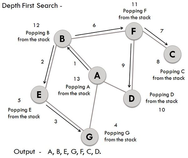
# Expected Output: 'A B D G E F C'

Depth-First Search (DFS) is a graph traversal algorithm that's simpler and often faster than its breadth-first counterpart (BFS). While it might not explore all vertices, DFS is still fundamental to numerous graph algorithms.

1. Initialize: Select a starting vertex, mark it as visited, and put it on a stack.
2. Loop: Until the stack is empty, do the following:
   • Remove the top vertex from the stack.
   • Explore its unvisited neighbors and add them to the stack.
3. Finish: When the stack is empty, the algorithm ends, and all reachable vertices are visited.

Here is the Python code:

def dfs(graph, start):
    visited = set()
    stack = [start]
    
    while stack:
        vertex = stack.pop()
        if vertex not in visited:
            visited.add(vertex)
            stack.extend(neighbor for neighbor in graph[vertex] if neighbor not in visited)
    
    return visited

# Example graph
graph = {
    'A': {'B', 'G'},
    'B': {'A', 'E', 'F'},
    'G': {'A'},
    'E': {'B', 'G'},
    'F': {'B', 'C', 'D'},
    'C': {'F'},
    'D': {'F'}
}

print(dfs(graph, 'A'))  # Output: {'A', 'B', 'C', 'D', 'E', 'F', 'G'}

BFS and DFS are both essential graph traversal algorithms with distinct characteristics in strategy, memory requirements, and use-cases.

1. Search Strategy: BFS moves level-by-level, while DFS goes deep into each branch before backtracking.
2. Data Structures: BFS uses a Queue, whereas DFS uses a Stack or recursion.
3. Space Complexity: BFS requires more memory as it may need to store an entire level ($O(|V|)$), whereas DFS usually uses less ($O(\log n)$ on average).
4. Optimality: BFS guarantees the shortest path; DFS does not.

Here is the Python code:

# BFS
def bfs(graph, start):
    visited = set()
    queue = [start]
    while queue:
        node = queue.pop(0)
        if node not in visited:
            visited.add(node)
            queue.extend(graph[node] - visited)
            
# DFS
def dfs(graph, start, visited=None):
    if visited is None:
        visited = set()
    visited.add(start)
    for next_node in graph[start] - visited:
        dfs(graph, next_node, visited)

Given an undirected graph, the task is to determine whether or not there is a path between two specified vertices.

The problem can be solved using Depth-First Search (DFS).

1. Start from the source vertex.
2. For each adjacent vertex, if not visited, recursively perform DFS.
3. If the destination vertex is found, return True. Otherwise, backtrack and explore other paths.

• Time Complexity: $O(V + E)$
  $V$ is the number of vertices, and $E$ is the number of edges.
• Space Complexity: $O(V)$
  For the stack used in recursive DFS calls.

Here is the Python code:

from collections import defaultdict

class Graph:
    def __init__(self):
        self.graph = defaultdict(list)

    def add_edge(self, u, v):
        self.graph[u].append(v)
        self.graph[v].append(u)

    def is_reachable(self, src, dest, visited):
        visited[src] = True

        if src == dest:
            return True

        for neighbor in self.graph[src]:
            if not visited[neighbor]:
                if self.is_reachable(neighbor, dest, visited):
                    return True

        return False

    def has_path(self, src, dest):
        visited = defaultdict(bool)
        return self.is_reachable(src, dest, visited)

# Usage
g = Graph()
g.add_edge(0, 1)
g.add_edge(0, 2)
g.add_edge(1, 2)
g.add_edge(2, 3)
g.add_edge(3, 3)

source, destination = 0, 3
print(f"There is a path between {source} and {destination}: {g.has_path(source, destination)}")

Given a directed graph and two vertices $src$ and $dest$, the objective is to print all paths from $src$ to $dest$.

1. Recursive Depth-First Search (DFS) Algorithm in Graphs: DFS is used because it can identify all the paths in a graph from source to destination. This is done by employing a backtracking mechanism to ensure that all unique paths are found.

2. To deal with cycles, a list of visited nodes is crucial. By utilizing this list, the algorithm can avoid revisiting and getting stuck in an infinite loop.

• Time Complexity: $O(V + E)$

  • $V$ is the number of vertices and $E$ is the number of edges.
  • We're essentially visiting every node and edge once.

• Space Complexity: $O(V)$

  • In the worst-case scenario, the entire graph can be visited, which would require space proportional to the number of vertices.

Here is the Python code:

# Python program to print all paths from a source to destination in a directed graph

from collections import defaultdict

# A class to represent a graph
class Graph:
    def __init__(self, vertices):
        # No. of vertices
        self.V = vertices

        # default dictionary to store graph
        self.graph = defaultdict(list)

    def addEdge(self, u, v):
        self.graph[u].append(v)

    def printAllPathsUtil(self, u, d, visited, path):
        # Mark the current node as visited and store in path
        visited[u] = True
        path.append(u)

        # If current vertex is same as destination, then print current path
        if u == d:
            print(path)
        else:
            # If current vertex is not destination
            # Recur for all the vertices adjacent to this vertex
            for i in self.graph[u]:
                if not visited[i]:
                    self.printAllPathsUtil(i, d, visited, path)

        # Remove current vertex from path and mark it as unvisited
        path.pop()
        visited[u] = False

    # Prints all paths from 's' to 'd'
    def printAllPaths(self, s, d):
        # Mark all the vertices as not visited
        visited = [False] * (self.V)

        # Create an array to store paths
        path = []
        path.append(s)

        # Call the recursive helper function to print all paths
        self.printAllPathsUtil(s, d, visited, path)

# Create a graph given in the above diagram
g = Graph(4)
g.addEdge(0, 1)
g.addEdge(0, 2)
g.addEdge(0, 3)
g.addEdge(2, 0)
g.addEdge(2, 1)
g.addEdge(1, 3)

s = 2 ; d = 3
print("Following are all different paths from %d to %d :" %(s, d))
g.printAllPaths(s, d)

A bipartite graph is one where the vertices can be divided into two distinct sets, $U$ and $V$, such that every edge connects a vertex from $U$ to one in $V$. The graph is denoted as $G = (U, V, E)$, where $E$ represents the set of edges.

You can check if a graph is bipartite using several methods:

BFS is often used for this purpose. The algorithm colors vertices alternately so that no adjacent vertices have the same color.

Here is the Python code:

from collections import deque

def is_bipartite_bfs(graph, start_node):
    visited = {node: False for node in graph}
    color = {node: None for node in graph}
    color[start_node] = 1
    queue = deque([start_node])

    while queue:
        current_node = queue.popleft()
        visited[current_node] = True

        for neighbor in graph[current_node]:
            if not visited[neighbor]:
                queue.append(neighbor)
                color[neighbor] = 1 - color[current_node]
            elif color[neighbor] == color[current_node]:
                return False

    return True

# Example
graph = {'A': ['B', 'C'], 'B': ['A', 'C'], 'C': ['A', 'B', 'D'], 'D': ['C']}
print(is_bipartite_bfs(graph, 'A'))  # Output: True

A graph is not bipartite if it contains an odd cycle. Algorithms like DFS or Floyd's cycle-detection algorithm can help identify such cycles.