Enhanced Spatial-Temporal Interpretable Deep Learning Model

SOPINet is a simultaneous Ozone and PM2.5 inversion deep neural Network. This tutorials contains how to configure the SOPINet model locally and help you to quickly use the model. In addition, we detailed how to adjust the parameters, which will help you get an optimized model of your own data.

Example Data Link: https://zenodo.org/record/7815394

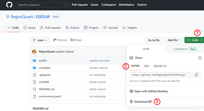
All of our source codes are tested in python 3.9/3.10 for both Win10 /11 and Ubuntu 20.04. You can used git clone to capture our code or directly download the zip file from our GitHub project page (https://github.com/RegiusQuant/ESIDLM). Here we show the two approaches respectively with vscode.

Installation method 1
Open the vscode and create a new folder, then you can clone the GitHub repository by the follow command:

git clone https://github.com/RegiusQuant/ESIDLM.git

Installation method 2
Download the zip file to your local at our project homepage ( https://github.com/RegiusQuant/ESIDLM) and unzip to the folder where you want.

We have listed all of the required packages of our model in environment.yaml file. You can try to configure in your existing environment one by one or create a new environment automatically by conda (recommend). Here we showed the second approach in our guide.

Setting environment method 1
Enter to the created folder firstly and used the follow code to build the required python packages (It is worth highlighting that you should have the conda software before). You can also set the name of your environment by replace myenv.

conda env create -f environment.yaml --name myenv

Setting environment method 2
Additionally, Mamba-forge install are also recommend in our tutorials. It will helps to speed up installation and improve installation stability. You should used the follow command to install mamba.

conda install mamba -n base -c conda-forge

Then, the installation command is the same as conda, just replace conda with mamba, as shown below:

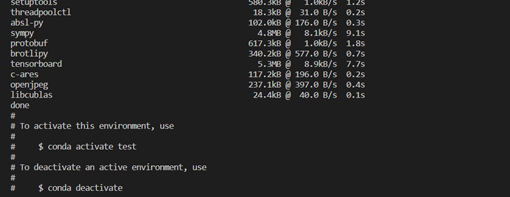
mamba env create -f environment.yaml --name myenv

When the environment is established well, you will see the following figure.

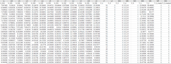
The data used for SOPiNet have two parts. The first part is the labeled data for modeling and they should be in .csv format and be named after train.csv, valid.csv and test.csv for training, validation and testing data, respectively. The second part is the unlabeled data for retrieval PM2.5 and Ozone of full image, which can be any name in .csv format and usually named by its date The format in each .csv should be as follows. To make the structure of data clearer, we set the continuous variables start with X_* and * should be in the sequence of number. The categorical variables should start with C_* and * should also be in the sequence of number. For the labeled data, it should be contain both PM2.5 and Ozone in-situ measurement for training and we default it with Y_1 and Y_2. In addition, to utilize more training samples, we used mask columns to deal with the absence of observations at those sites. The main structure of data is as follow:

After you finished the installation of the model, you will see the following main folder in the project(esidlm, examples, outputs). All of the codes are encapsulated in the esidlm folder and we do not recommend you change the code in this folder. In the examples folder, we uploaded a small part of train/valid/test data and the “SOPiNet.ipynb” file in this folder is showed how to used esidlm module as an instance. You only need to change some simple parameter configurations and run each cells in the jupyter notebook by order to get your own model. To simplify use, we have consolidated all configurations into a dictionary variable SOPINET_TRAINING_ CONFIG. Then we will briefly explain what you need to modified in your local.

Basic Parameter Configuration
Global

• seed: the random seed in model. (default=42).
• output_folder: This parameter control output path of the model after training, we default it to "../outputs/sopinet"

Data

• train_data: the file path of your train data. (default=’ ../data/sopinet/train.csv’) valid_data: the file path of your valid data. (default=’ ../data/sopinet/valid.csv’)
• test_data: the file path of your test data. (default=’ ../data/sopinet/test.csv’)
• cont_cols: the columns name of continuous variable in the train data. In our study, we default it to “X_1, X_2 ‧‧‧‧‧‧X_n” but it can be flexible.
• cate_cols: the columns name of categorical variable in the train data. In our study, we default it to “C_1, C_2 ‧‧‧‧‧‧C_n” but it can be flexible.
• time_cols: the columns of time series variable in the train data. Compare to cont_cols, we processed them into transformer frame. Noticed that each different time period in the time series needs to be in the list independently. For example, If you have three days of time series data of meteorological data (RH,WS,PS). The time_cols should be the format as follow:

time_cols = {
    [RH_1, WS_1, PS_1],
    [RH_2, WS_2, PS_2],
    [RH_3, WS_3, PS_3],
} 

• target_cols: the columns name of prediction in train data. Due to the ability of simultaneous inversion, it should be set two predictions name. In our study, we default it to “Y_1, Y_2” but it also can be flexible.
• mask_cols: the columns name of you want to masked in targets value. The masked value will not participate in the calculation of the loss function. In our study, we masked the in-situ measurement which are missing. Note that code used 0 or 1 to determine whether the value mask or not.(1 = keep, 0 = mask) and the order should be same with target_cols.
  
  

Hyperparameter configuration
Dataloader

• batch_size: The number of data samples captured in one step training.(default=64)
• num_workers: the number of process created when used dataloader. (default=4)

Model

• d_embed: the number of dimensions used to represent each input feature in the embedding for categorical. (default=32)
• d_model: the number of hidden layer nodes. (default=256)
• n_layers: the number of hidden layer. (default=1)
• n_head: the number of attention heads used in the multi-head attention mechanism. (default=4)
• p_drop: the percent of neurons are temporarily removed from the network during training. (default= 0.3)
• act_fn: Activation function. (default= relu)
• lr: learning rate. (default= 3e-4)
• weight_decay: the value for penalizes large weights in the model during training to prevent overfitting. (default= 1e-5)

Model_Callback

• save_top_k: specifies the number of best models to keep based on a given metric during training on validation accuracy. (default=1,save the best)
• monitor: specifies the metric to monitor during training.(default=valid_loss) Mode: specifies whether the monitored metric should be minimize(MAE) or maximized (R). (default=min)
• verbose: determines whether to print information about the saving process to the console. (default= True)
• patience: specifies the number of epochs to wait for improvement in the monitored metric before stopping training.( default=10)

Trainer

• max_epochs: specifies the maximum number of epochs to train for.( default=5)
• accelerator: specifies the hardware accelerator to use during training (default=”gpu”)
• devices: specifies the number of devices to use during training. (default=1)
• deterministic: ensures reproducibility of the training results. (default=True)
  
  

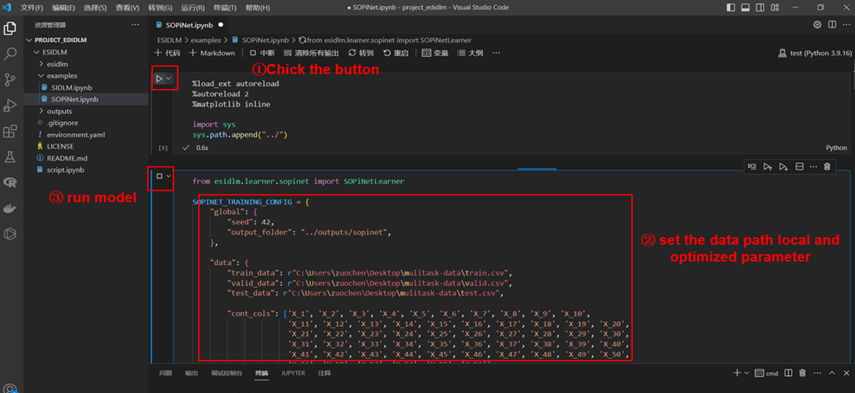
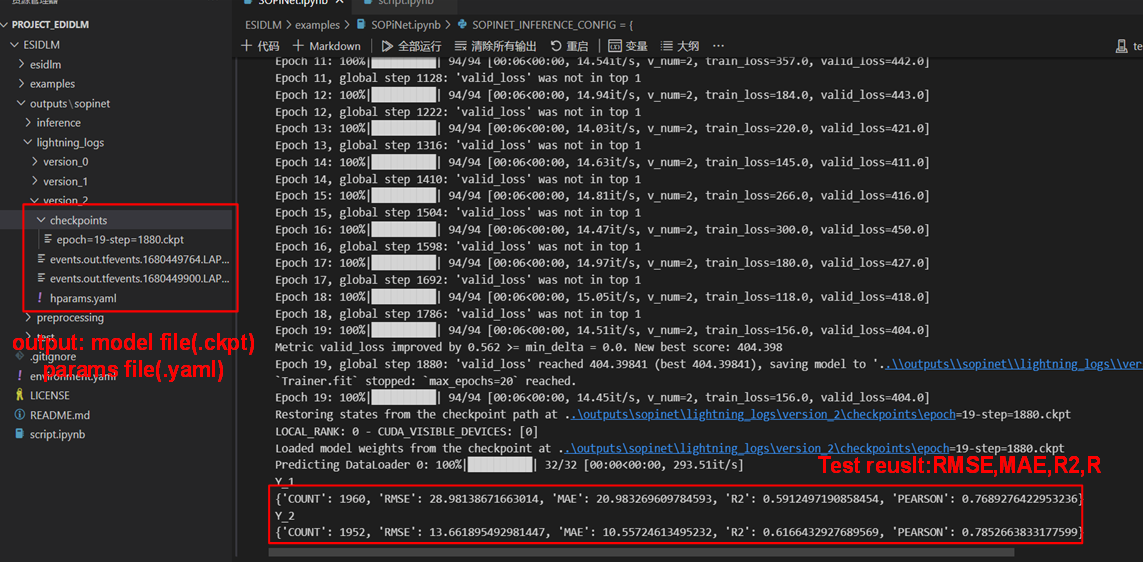
Here, we showed a complete training process using example train data. First, open the ESIDLM project and change the system path by sys (first code cell), then set your own data path and optimized parameter. After setting the parameters well, you can create a SOPiNetLearner object and call run_model_training function.

In this instance, we set the parameter with "batch_size": 64, "d_embed": 32,"d_model": 128,"n_layers": 1,"n_head": 4,"p_drop": 0.1. As you can see, just after 20 epoch of training (2 minute), we have achieved remarkable accuracy with 0.59 R2 of PM2.5 (Y_1) and 0.61 R2 of ozone (Y_2). Now, a full round of training model is finished, the rest need to constantly adjust the parameter and optimize the model.

It should be emphasized that both each training of the model and Hyperparameter file are saved in the output folder (default=’ /.. /outputs/sopinet’).

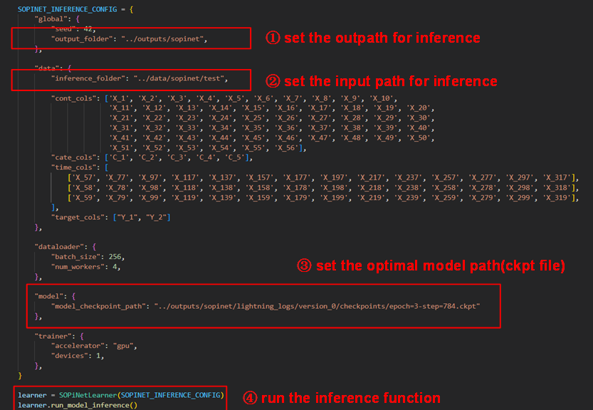
After determining the best optimal model, we will use this model for inference. It is also should used the dictionary named SOPINET_ INFERENCE_CONFIG to which is mostly similar to the training model. As follow, you should set the input and output folder in which the input data should be unlabeled. Then set the optimal model path and run the inference function.

SIDLM is under construction.