1. hubbard_functions.py : Contains all the functions programmed and used for solving one-dimensional hubbard model. It includes numpy based functions to : calculate the dimension, set basis states for the system, hamiltonian of the subspace and the fock space for a given N (number of lattice sites and electron occupancy (r)). It also conatns functions which generates the hamiltonian of the system in temrs of spin operators and some functions are to study some properties of the system for example the density of states and site occupation fo eigenstates.
2. hubb0_properties, hubb2_properies : Contains some visuals which explain the properties of the hubbard model with 1 and 2 allowed spins respectively at each site.
3. VarQITE Results : Contains the solutions for Variational Quantum Imaginary Time Evolution for different ansatz. It also contains the companrison results and the overall performance of the algorithm for one-dimensional hubbard model for 2 to 8 lattice size. ===================================================================================

In this project, we study lattice models like Tight Binding Model, Hubbard Model. We generate matrices of these models, solve them using NumPy and discuss some of the properties of the eigenvalues and eigenvectors. We realize the need of quantum simulation of these models and propose a quantum method for solving them. We implement it on a quantum circuit in different ways and compare the solutions with the NumPy results.

The Tight Binding Model describes the electronic structure of solids by considering the onsite energies and hopping energy of electrons.

$$ H_{\text{sys}} = \sum_{i} \epsilon_i c_{i }^{\dagger} c_{i } + t \sum_{i } (c_{i}^\dagger c_{(i+1) } +h.c. ) $$

Here, $c^\dagger_{l}$ is the creation operator which creates an electron at site l. On exact, diagonalization using discrete fourier transform, we find out that the eigenvalues follow the cos function.

$H_{\text{sys}} = \sum_{k } (\epsilon + 2 t \cos{\frac{2 \pi k}{N}}) c^\dagger_{k } c_{k }$

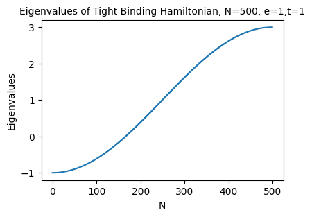
We create the matrices for one electron occupation Tight Binding Model and solve it using NumPy. Using the eigenstates obtained from solving the mkatrix, we find the occupation of that eigenstate at all the lattice sites and plot the probability of the state occupying the sites. In the following figures we show how different onsite energies result in different occupation of the ground state (vec 0) and the eigenstate with maximum energy (vec 1).

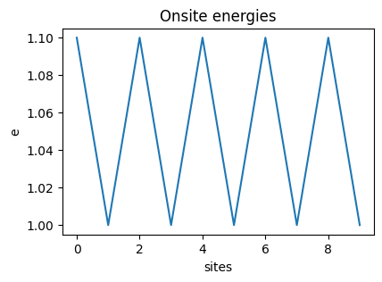
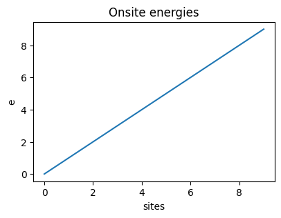
e peak	e periodic	e increasing
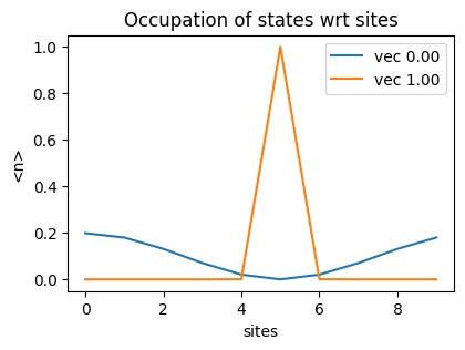
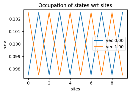
occupation peak	occupation periodic	occupation increasing

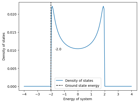
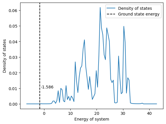
It is used to understand the energy distribution in a system. We find this using a delta or a lorentzian function. Once we have the eigenvalues of a system, we can find the distribution of these eigenvalues across an energy range. We can use the Lorentzian function along with the delta function to plot the density. The Lorentzian function broadens the delta function peaks corresponding to individual energy level giving a continuous density plot.

The following figure gives the Density of states for N=100, number of centers = 150, gamma = 0.3, t=1 and e=[0]*N

$$ D(\omega )= \sum _k \delta (\omega - \epsilon _k)$$

N site lattice model, with only one allowed spin. Describes the electronic structure of a solid by considering the onsite, hopping and nearest neighbour interaction term.

$$H = \sum_i \epsilon _{i} c^\dagger _{i} c _{i} + t \sum _{i} (c^\dagger _{i} c _{i+1} + h.c.) + U \sum _{i} n _{i} n _{i+1}$$
We now write a generalised matrix for a Hubbard model. This can now handle any electron occupation. It takes the description of the lattice model adn the number of electorns as input and returns the Hamiltonian matrix of that subspace. For an N site lattice model and r occupied electron, the dimension of the Hamiltonian becomes $^NC_r$. The sum of all such dimensions is $2^N$ which is the dimension of the whole fock space. One can divide the fock-space problem into these subspace problems and solve each of them individually to extract more information about the fock-space.

In the following figures, we solve a 12 site Hubbard Model with $\epsilon _k = 1$, t=1 and U=1. We solve it for different electron occupation and find the eiegenstate occupation.

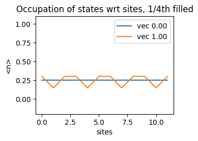
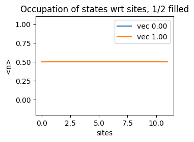
1 electron	1/4th occupation	1/2 occupation
1 Hole	3/4th occupation

In the following figures, we solve a 12 site Hubbard Model with $\epsilon _k = 1$, t=1 and U=1. We solve it for different electron occupation and find the density of states.

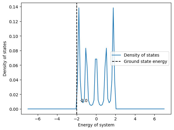
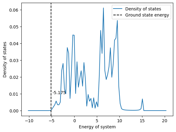
1 electron	1/4th occupation	1/2 occupation
1 Hole	3/4th occupation

We conclude from above data that a lattice problem with r-electron is the same as a problem with r holes. Their eigenvalues, eigenstates, their site occupation and the density of states have similar trends.

$$ H = t \sum_{j, \sigma} (c^\dagger_{j , \sigma} c_{j+1, \sigma } + c^\dagger_{j+1, \sigma} c_{j \sigma}) + U \sum_j n_{j \uparrow} n_{j \downarrow} $$

For one orbital models with two allowed spins, the fock dimension is exponentially larger than fock dimension of spinless models. While spinless one orbital model has $2^n$ dimension, the full model has $4^n$ dimensions. We can see how the dimension for the two models increases in the first figure below.

spinless vs 2-spin fock dimension

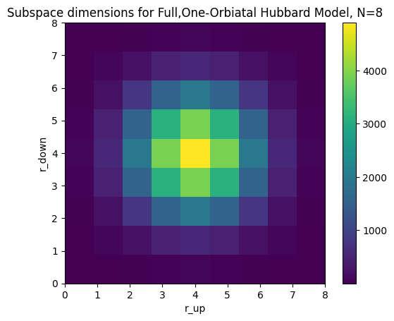
hubb2 sub dimensions

For each combination of up and down electrons, the model will have a subspace of a specific dimension. We can see how the subspace dimension varies with number of up and down electrons in the second figure above.

We can solve a lattice model effectively by breaking down the problem into its subspces and solving them using NumPy. However, as the number of sites increases, the dimension of subspaces increase and the time taken to generate their basis and then generate the Hamiltonian becomes exponentially larger.

Fock dim vs N

Sub dim vs N

Basis time vs N

In the above figures we can see how the fock space dimesnion increases exponentially, how the subspace dimesnion is maximum for half-filled electron and how that number increases appreciably with increasing lattice size. We can also see how the time taken to generate the half-filled basis increases exponentially with increasing lattice size.

We will first discuss ways in which we can implement the lattice model hamiltonian on a quantum circuit. There are different transformations that we can do to change a fermionic operator to a spin operator. We disscuss one such transformation.

So far, we were representing and solving the tight binding hamiltonian in terms of the fermionic creation $c^{\dagger} _j$ and annihilation $c_j$ operators. To be able to implement this on a quantum computer, we need to convert it into a spin problem. Jordan-Wigner transformation maps these operators to spin operators that we can eventually implement on quantum computers in the forms of quantum gates. We will use the following mapping strategy to do the same :

$$c^{\dagger} _j = \frac{X_j-iY_j}{2}$$

$$c_j = \frac{X_j+iY_j}{2}$$

To preserve the anticommutation relations ($\lbrace \hat{c}^\dagger _\alpha, \hat{c}^\dagger _\beta \rbrace=0$$) of the fermionic operators, Z gates are added to add phase to the spin operators.

$$c^{\dagger} _j = Z^{\otimes (j-1)} \otimes \Big( \frac{X-iY}{2} \Big) _j \otimes I^{\otimes (N-j)} $$

$$c _j = Z^{\otimes (j-1)} \otimes \Big( \frac{X+iY}{2} \Big) _j \otimes I^{\otimes (N-j)} $$

On using this transformation on our fermionic Hamiltonian, we get the following spin Hamiltonian :

$$ H _{JW}= \sum _k \epsilon _k \Big( \frac{\textbf{I}-Z}{2}\Big)_k + t \sum _k \frac{X _k X _{k+1} + Y _k Y _{k+1}}{2} + U \sum _{k=1}^N \Big( \frac{\textbf{I}-Z}{2}\Big) _k \Big( \frac{\textbf{I}-Z}{2}\Big) _{k+1} $$

As this expression is expressed in terms of the Pauli operators, we can implement this as a gate in a quantum circuit.

One can use imaginary time evolution to find the ground state and energy of a Hamiltonian. A state $| \psi \rangle$ of the system can be written as : $| \psi \rangle = \sum _i c_i |b _i\rangle$, where $|b_i\rangle$ are the basis states of the system and $c_i$ are complex amplitudes. On applying the time evolution operator , $U | \psi \rangle =e^{-H\tau} |\psi \rangle$, we get :

$e^{-H \tau} | \psi \rangle = e^{-E_0 \tau} [c_0 |b_0 \rangle + e^{-(E_1-E_0) \tau} c_1 |b_1 \rangle +....+ e^{-(E_{n-1}-E_0) \tau} c_{n-1} |b_{n-1} \rangle] $

One can see that for $\tau \xrightarrow{} \infty$, all the other coefficients tend to zero and we are left with the ground state $|b_0 \rangle$.

We use a variational quantum algorithm (VQA) to implement imaginary time evolution. We make use of the VarQITE (Qiskit) time evolution algorithm and input an evolution problem defined using the lattice Hailtonian. The varitional algorithm takes a parameterized ansatz as input and finds a set of parameters which minimizes the expectation value of the Hamiltonian. It is therefore important to take an ansatz which spans all the wavefunctions and can be trained efficiently. In the following sections we try out two different ansatz, compare it to the benchmarked SciPy and classical results.

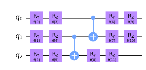
When enough information about the interested eigenstate is not known, a heuristic ansatz that is arbitrarily parameterized and entangled, can be used, such as Efficient SU(2) ansatz. Here is a circuit of this ansatz repeated once.

One can use the python package qiskit-symb, to see the parameterized state obtained from this circuit. One can also observe the amplitudes of different states in this statevector and modify their ansatz in order to achieve specific amplitudes for specific states.

We compare the efficiency of SU(2) VarQITE method with the SciPy method. This solves the application of the time evolution operator for imaginary time on the quantum state at all the discrete steps. The following figures show the comparison of performance of SciPyImaginaryEvolver and VarQITE with SU(2) ansatz.

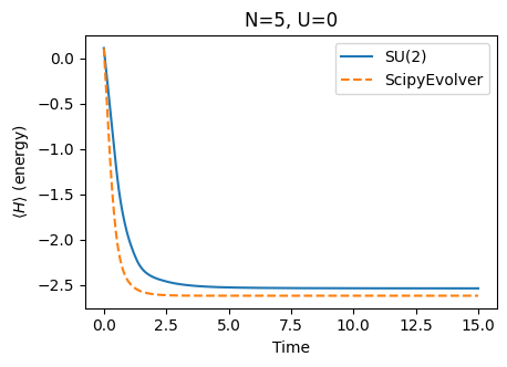
Estimated eigenvalues during time evolution

Accuracy Comparison

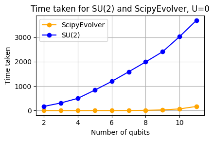
Time Comparison

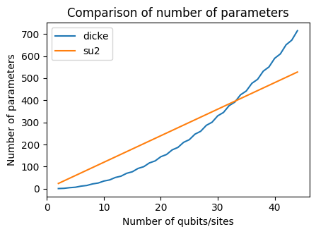
We use the circuit to create Dicke states, which are superposition of states with equal weights, and parameterize it to form our ansatz.

We can see from the comparison below that the number of parameters required for it less than number of parameters required for SU(2) repeated thrice.

We use this ansatz for solving different subspaces of our Hamiltonian. The results and the properties we study are mentioned in the following section. We plot the performance of the quantum method, the numpy method the the scipy method for two different values of U.

In this section we make use of the information we received from the variaitiona method and see which properties we can study using these results.

In this section we study how the energy of the system varies as the interaction increases.

We can see that as U increases for a certain model with certain number of lattice sites, the energy of the system increases. We can also see that the lowest energy of a system is for the half-filled scenario when there is no interaction present. As the interaction increases, the lowest energy shifts to the cases where the electron occupation is less.

We find the density of states from the eigenvalues we obtained from the variational method and we compare it with the density of states we get from the eigenvalues calculated from numpy.

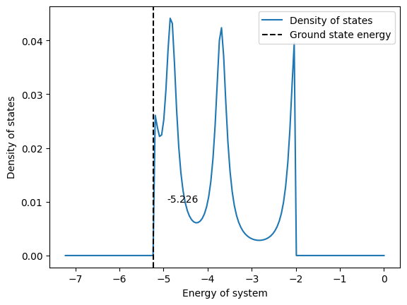
DOS NumPy

DOS VarQITE

We can see that the results we got, give a similar trend for density states. However, the values calculated are not very accurate and thus the figure is shifted from the original points. However, this is good to understand the distribution of eigenvalues over an energy range.