Light version of this Research Paper co-authored with Emilie Géraud.
Air pollution is a world major issue which inflicts many damages. This study takes place in Lille in France and attempts to forecast PM10, ozone and nitrogen dioxide for up to 48 hours. These three pollutants are known for their harmful effects on human health. A solid forecasting system will allow to predict the air pollutant concentration, essential for information and alert thresholds set by European Directive 2001/81/CE, and thus to set up action plans to avoid and limit health risks. Hourly data collected since 2013 in Lille stations, combined with weather historical data, have been used for different forecasting methods: Multiple Linear Regressions, Recurrent Neural Networks, Sequence to Sequence models and Convolutional Neural Networks. The main objective is to forecast the air pollutants concentrations for up to 48 hours. The results obtained using these five methods show that, overall, Sequence to Sequence models provide the best forecasting models. We also compared the most precise process between the prediction of three pollutants with a model and three independents models predicting a unique pollutant.
Many air pollutants are known to have adverse effects on the environment and human health. They can, in fact, act on the nervous, respiratory, cardiovascular or hormonal systems. A World Health Organization (WHO) study has counted 2 million premature deaths per year due to diseases caused by air pollution. Among the known air pollutants, three were chosen to carry out this study. These are Particulate matter 10 (PM10), ozone (O3) and Nitrogen dioxide (NO2). PM10 is airborne particulate matter with an aerodynamic diameter of less than 10 µm. They are mainly generated by transport, energy production, and industrial and agricultural activities. NO2 belongs to the family of nitrogen oxides (NOx) and mainly comes from road traffic and heating. Finally, O3 is formed by chemical reactions from pollutants such as NOx or hydrocarbons.
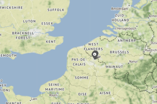
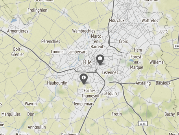
Our study is based on data measured at the Lille Fives station (located to the East of Lille) and at the Wattignies station (in the South of Lille). The Lille Fives station is an urban background station located in a densely populated area and the Wattignies station is a peri-urban background station located on the outskirts of Lille. They are therefore representative of “urban” ambient air quality without targeting the impact of a particular emission source. The Lille Fives station measures NO2 and PM10 concentrations and the Wattignies station measures O3 concentrations.
The data used for this study are hourly samples between January 1, 2013 01:00 and October 05, 2020 00:00 (N = 68,015) and concern the following pollutants: PM10, O3 and NO2. These are hourly concentrations measured in
About 5% of the dataset was missing, mainly because of the maintenance of the measuring devices. In addition, those missing values were usually successive for a long range (sometimes a week long). To fill these gaps, we used values from nearby stations. Between two stations we made a linear regression to find the function that best approximate the relation between the measurements, we filled those estimated values with two or three nearby stations, and we completed the last missing values with linear interpolation.
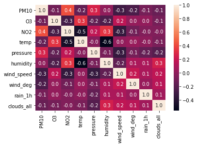
If r, the correlation factor, is close to 1 (or -1), it means it exists a positive (or negative) linear relation between the two variables. In return, if r is near 0, it means it does not exist a strong linear relation.
In terms of weather variables, the strongest positive correlation is between PM10 and pressure (0.26) and the strongest negative correlation is between PM10 and wind speed (-0.29). These correlations are explained by the fact that PM10 occurs during anticyclonic conditions. These conditions are characterized, in part, by high ground pressure and weak or no wind, which boost the accumulation of particles. The low wind speed does not allow a horizontal dispersion of particles. Similarly, ozone has a correct positive correlation with temperature (0.33). Indeed, ozone is formed in the presence of UV radiation and high temperature. Concerning nitrogen dioxide, it has his highest positive correlation with humidity (0.33) and his lowest negative correlation with temperature (-0.46) and wind speed (-0.34). As with particles, nitrogen dioxide has high concentrations in anticyclonic conditions, which explains its correlation coefficient with wind speed. In relation to its coefficients with humidity and temperature we will see later that this is due to its correlation with ozone.
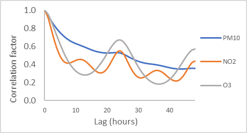
The autocorrelation of the three pollutants shows that the concentration of each pollutant is highly correlated with the concentration of the same pollutant a few hours earlier. This is especially true for PM10. The models used to predict the concentrations of PM10, O3 and NO2 will be better when they predict the concentrations of these pollutants shortly in advance (0 to 4 hours). Moreover, it would seem that models can also have interesting results when they predict ozone and nitrogen dioxide concentrations 24 hours ahead, as the linear correlation coefficient is relatively stronger 24 hours ahead for these two pollutants.
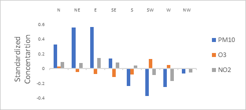
On average, a higher concentration when the wind comes from the Northeast and the East. We know that once deposited on the ground, particles can be re-suspended in the air under the action of the wind. It has been shown that particles can be transported very far by the wind, as shown by an Airparif study indicating that in an average situation in the Paris agglomeration, 70% of the particles come from other French or European regions. Here the high concentrations of particles are observed when the wind comes from the Northeast or from the East, it could then be the particles coming from the metropolis of Brussels located 93 km (as the crow flies) from Lille. This metropolis is, indeed, much closer to Lille than the metropolis of Paris (204 km) which would explain why the high concentrations come from the Northeast / East.
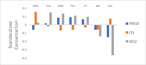
These high PM10 concentrations are also observed from Tuesday to Friday, i.e. during the week. As the particles are mainly emitted by vehicles and domestic heating, these concentrations can be explained by the more intense traffic during the week than on weekends. This is especially true at the level of large cities such as Lille.
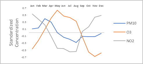
Looking at the variable of the months of the year, high concentrations are observed between December and May, i.e., in winter and spring. The episodes of particulate pollution in winter are due to vehicle and domestic heating emissions combined with strong anticyclonic conditions preventing the dilution of particles. Spring episodes are due to other sources such as ammonia from agricultural activities, which, combined with nitrogen oxides from vehicle emissions, can form particulate matter. Because ozone is formed with solar ultraviolet radiation and high temperatures, we observe higher concentration during the warm months. It is also the reason why ozone has higher concentrations during the day than during the night (~20% difference in average). In return, we observe that concentrations of NO2 are higher in the cold month. With lower temperatures and reduced UV radiation, NO2 does not transform into ozone, which explains its high concentrations.
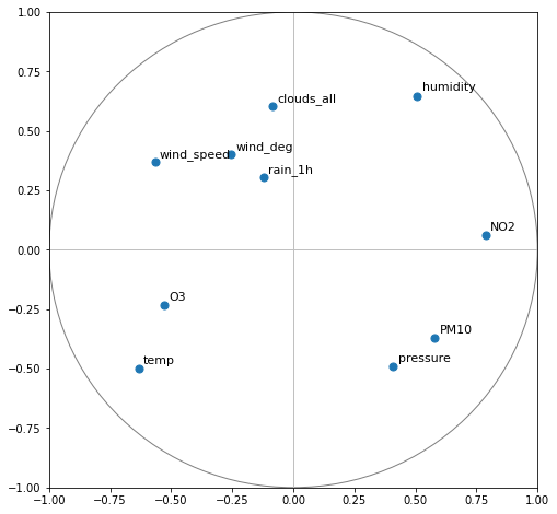
Principal Component Analysis (PCA) is an operation that project the data on the most significant vectors. The core idea is to calculate the eigenvalues and their associate vectors of the correlation matrix. For visualization purposes, we plotted the plane generated by the 2 largest eigenvalues (called F1 and F2). This formatted plane allows to retain 42% of the variance. The correlation circle shows the relation between the variables. Grouped variables are positively correlated and if they are far from the origin, it means they have a good representation in the hyperplane.
As seen previously, PM10 and NO2 appear globally under the same conditions of pressure, temperature and wind speed which may explain this strong correlation between the two pollutants.
It exists a strong negative correlation between ozone and nitrogen dioxide (confirmed by the correlation circle). Indeed, the NO2 is transformed into ozone thanks to the dioxygen in the air, which explains why an increase in the ozone concentration results in a decrease in the NO2 concentration.
A concurrent reaction can also occur in heavily polluted areas and under certain insolation conditions, high concentrations of nitrogen monoxide can lead to the nightly destruction of ozone, this is the titration effect.
As a result of these two reactions, but especially as a result of the first one occurring more frequently, high ozone concentrations are observed at low nitrogen dioxide concentrations and vice versa. This explains why NO2 is more concentrated in autumn/winter and why NO2 has a strong positive correlation with humidity and a strong negative correlation with temperature.
In order to select the explanatory variables that are part of the MLR models we used a method called backward selection. This method starts with all candidate independent variables in the model. At each step, the variable that is the least significant is removed. This process continues until no non-significant variables remain. Here the significance level at which variables can be removed from the model is a p-value greater than or equal to 5% (p-value ≥ 0,05), depending on the t-test. In our study, we use this method in order to obtain a model for each pollutant at t+Δt with Δt = 6, 12, 24 and 48 hours (12 models in total).
The input data is a matrix of shape (168,10) corresponding to the 168 previous time steps of the 10 features. The output is a vector of shape (48,3) corresponding to the 48 next time steps for the three pollutants. We also compared the accuracy between a model that predict the three pollutants and three independent models predicting each pollutant concentration. To make the difference we call this difference multi output and single output respectively.
To correctly compare the different proposed methods, we divided our dataset into three sub-datasets: training (70%), validation (15%) and test (15%). For each proposed method, a first step was to find the hyperparameters that best fit our model. To achieve this, we tried to vary parameters depending on the architecture like the number of units, the filter size, the dropout, normalization layer… The idea was to select the best model that best fit our data by analyzing the training curves. Then, we train over the whole dataset (training and validation datasets) with this best set of hyperparameters. In the result table, the score of each architecture corresponds to the performance score on the test set.
For all our architectures, we trained our models with 30 epochs and a mini batch size of 128. About the optimizer, we used RMSProp with a learning rate of 0.001. The loss function is Mean Square Error and the training has been realised on a Nvidia Tesla V100. For autoregressive methods we did not use the teacher forcing method.
To compare the accuracy of each architecture, we calculated performance score: Mean Absolute Error (MAE) and R² score. We look for the lowest MAE and the highest R² score . A negative R² means that the mean of the data provides better result than the predictor. An R² equal to 0 signifies that the predictor is as performant as the mean of the observed values. We chose to display the metrics for 4 different forecast hours: 6, 12, 24 and 48 hours.
MAE can be understood as the average difference between the predicted and the observed value while R² represents the proportion of the variance in the dependent variable that is predictable from the independent variable.
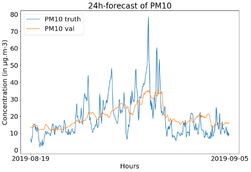
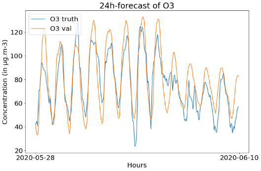
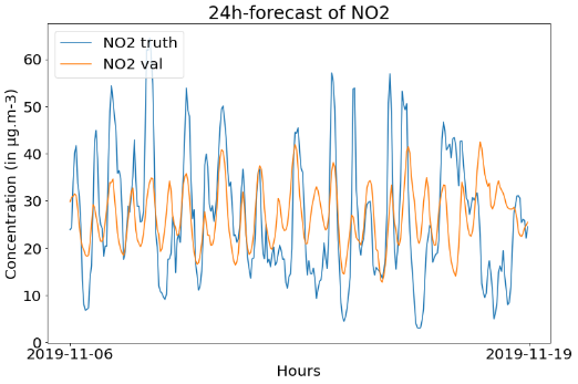
Example of results obtained with Seq2seq GRU with Luong Attention : PM10, O3 and NO2 forecasted at 24 hours vs their ground truth.
The previous study on autocorrelation is validated by the MLR models: the prediction models are more efficient for PM10 and NO2 at t+6h and for ozone at t+24h. Overall, we find the same orders of magnitude as in other studies.
In our benchmark, we observe that attention-based models show the best performances between the neural networks. Indeed, the sequence to sequence GRU with Luong attention is our best predictor and, for instance, accounts for up to 71.8% of the variance with the forecast of ozone at Δt = 6h.
The studied pollutants present different ranges of accuracy. The ozone seems easier to forecast because our predictors show better performance score. It is mainly due to the periodicity of the concentrations between the day and the night and makes it more foreseeable. Concerning the PM10, the accuracy strongly reduces with more distant forecast, which is also the case for the other pollutants, but their accuracies reduce more slowly. This difference is explainable by the non-time dependence of the particulate matter concentrations. As shown in the Time Series Analysis part with autocorrelation figure, we observe periodical correlation peak each 24h for ozone and NO2. As an addition, the variation of PM10 are slighter (low volatility) and short-term correlation (Δt < 12h) is much higher with PM10 than other pollutants and emphasizes the prediction goodness at short-term.
PM10 and O3 have better results with single output models while multi outputs seems more accurate with NO2. However, fine-tuning hyperparameters for each model and each pollutant was a complex process. Thus, for the future, a better methodology would be to compare proposed architectures with multi outputs models and finally train single output models.
We proposed a study to forecast air pollution concentration in Lille. The principal objective was to forecast for a range of 48 hours with the previous 168 time steps as an input. Pollutant concentrations have been completed with meteorological data. We first made a Time Series Analysis to understand our dataset, and then we applied Machine Learning methods. The comparison of the applied technique, with appropriate metrics, allows to present the Sequence to Sequence GRU-based with Luong Attention as the most performant model among our benchmark. During our study, we also investigate on the performance differences between multi and single outputs models. We conclude that, in our case, single outputs models are more accurate with the PM10 and ozone predictions but the process did not require to train these two types of models for each architecture.
In the future, we will work with more features like others stations samples, similarly to a network, in order to predict the pollution movements. The use of other air pollutant would be relevant because they have many interactions together in atmospheric processes Another interesting idea would be to add weather forecast to our dataset and increase the accuracy. Finally, traffic data would be a reliable dataset for this project. Adding more data will certainly improve the accuracy.
