Analysis of limited proteolysis small molecule mapping (LiP-SMap) data.
Data were prepared for analysis by concatenating input files, by gathering annotations for the organisms in question, and by performing a phylogenetic analysis. These data preparation steps were less prone to changes and updates compared to the analysis pipeline, and were therefore held separate.
Data were concatenated from the original source:
Rscript source/concatenate_input_data.R ${INDIR} ${OUTFILE}
Missing loci were amended by the concatenation R script with the intermediate files intermediate/missing_locus_uniprot_IDs.txt and intermediate/uniprot_locus_missing.tab.
The R script finally produced concatenated LiP-SMap in OUTFILE.
Additional annotations were downloaded from KEGG:
source/get_ko_and_modules.sh
...providing these annotation files:
data/KEGGgene_uniprot_organism.tab
data/KEGGgene_KO_organism.tab
data/KEGGgene_module_organism.tab
data/KEGGgene_EC_organism.tab
data/EC_description.tab
data/module_description.tab
data/module_compound.tab
data/module_reaction.tab
data/reaction_compound.tab
Orthologs in the organisms were identified via UniProt and the eggNOG labels:
source/identify_orthologs.sh
...resulting in these data files:
data/uniprot_eggNOG.tab
data/organism_uniprot.tab
The second file lists all UniProt sequences in the organisms, so that those without an ortholog could be accounted for as well.
Annotations for the eggNOG labels were acquired:
source/get_eggNOG_categories.sh
...and filtered with R:
source/filter_eggNOG_annotations.R
...thus producing the final eggNOG ortholog annotations:
data/eggNOG_annotations.tab
Gene identifiers were downloaded for the LiP-SMap organism proteins:
source/get_uniprot_gene_identifiers.sh
...producing these lists:
data/uniprot_gene.tab
data/uniprot_locus_complete.tab
A phylogenetic analysis was performed on Calvin cycle enzymes from the corresponding KEGG module (M00165), supplemented with transaldolase (K00616, K13810), triose-phosphate isomerase (K01803), and ribulose-phosphate epimerase (K01783). Sequences were downloaded from UniProt, filtered with CD-HIT, aligned with MAFFT, and used to make trees with FastTreeMP:
source/Calvin_cycle_phylogenetics.sh
Within the phylogenetic analysis script, the NCBI taxonomy was consulted to give organism labels to all proteins in the tree using the helper script source/taxid-to-taxonomy.py. Furthermore, UniProt sequences were acquired based on KEGG orthologs using the helper script source/uniprot_sequences_from_KO.sh.
Assessment of minimum q value correlation and agreement on significant interactions between repeated experiments was performed with this script:
source/dates.R
...yielding the following plots:
results/dates_min_q_cor.pdf
results/dates_agreement.pdf
A reduced dataset was prepared from the original source to be used in the tutorial. The reduced tutorial dataset consists of a subset of metabolites measured in most organisms, and a subset of 250 randomly selected proteins per organism. The proteins were selected to overlap in terms of ortholog groups in order to permit some of the analysis steps.
This script was used to subset the data from the original source:
source/tutorial_data.R
The tutorial dataset mimics the file names and directory structure of the original data and is thereby divided into one folder per organism, with one file per experiment (including repeated experiments), for example this file:
data/tutorial/lipsmap/Cupriavidus/comparisonResult_3PGA_7_grouped_annot_20200914.csv
A series of R scripts were used to test hypotheses, and to generate data visualizations and tables. All scripts can be run in order by invoking the analysis shell script:
./analysis.sh ${INFILE} ${OUTDIR}
...where INFILE is an output file from source/concatenate_input_data.R, and OUTDIR is a desired output directory, in which each script will have its own output subdirectory.
Standard output ("stdout") and standard error ("stderr") reporting from the scripts is logged in this file:
${OUTDIR}/analysis.log
The individual steps of the analysis are described below.
Metabolite interactions with enzymes and non-enzymes were compared using Fisher's exact test:
Rscript source/enzymes.R ${INFILE} ${OUTDIR}/enzymes
...yielding the following results:
Fisher_exact_test_for_enzyme_interactions.tab
Proteins were grouped by various functional categories (EC, GO, KEGG module, pathway) and tested for enrichment of interactions:
Rscript source/functions.R ${INFILE} ${OUTDIR}/functions
...yielding the following results:
Fisher_exact_test_for_EC_interactions.tab
Fisher_exact_test_for_GO_interactions.tab
Fisher_exact_test_for_module_interactions.tab
Fisher_exact_test_for_pathway_interactions.tab
Interaction patterns with orthologs were compared within and between organisms:
Rscript source/orthologs.R ${INFILE} ${OUTDIR}/orthologs
...producing a range of comparison plots and tables.
Overview and clustering of orthologs across the whole dataset:
orthologs_interaction_comparison.png
orthologs_interaction_clustering.pdf
metabolite_function_interactions.pdf
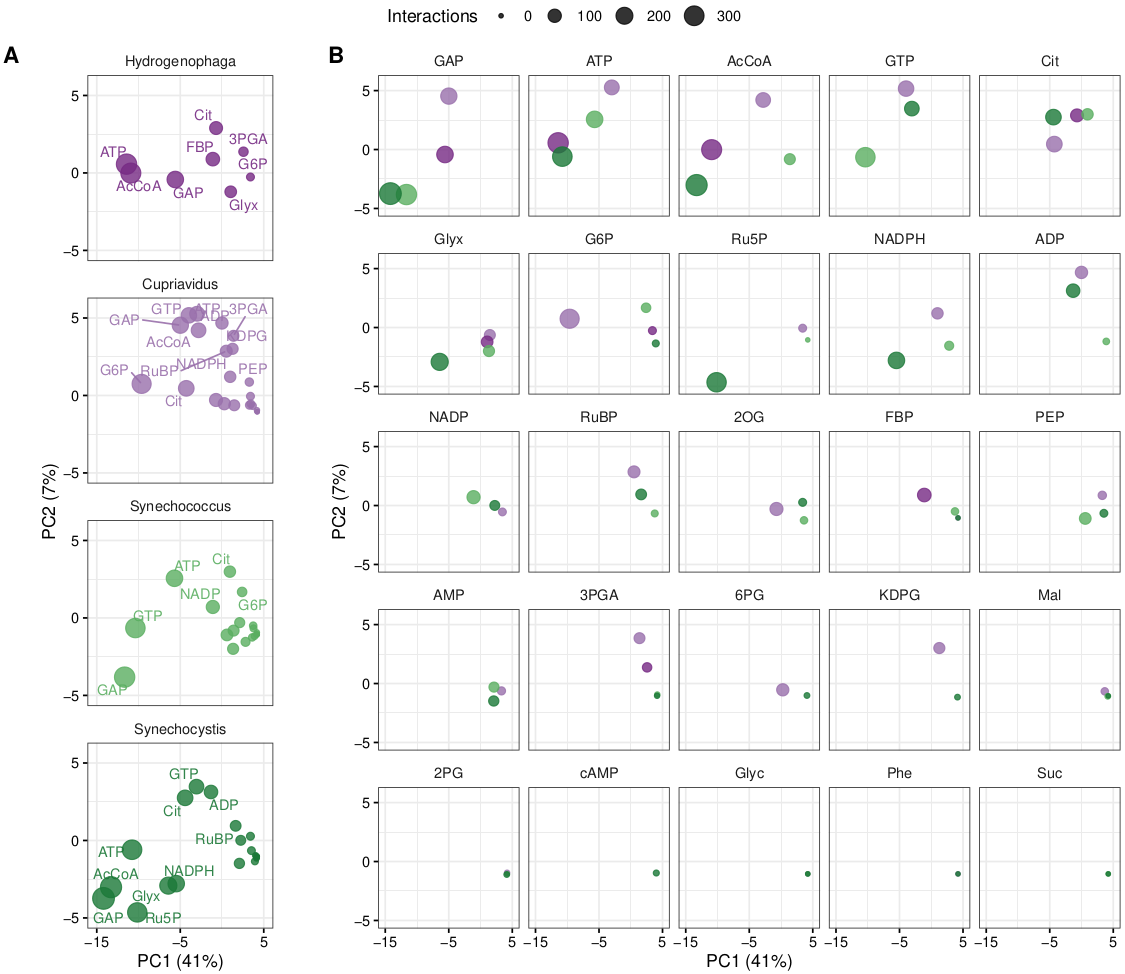
PCA analysis at high (Fig 1) and low concentration:
Fig.orthologs_interaction_pca.high.pdf
Fig.orthologs_interaction_pca.low.pdf
orthologs_interaction_pca.high.pdf
orthologs_interaction_pca.low.pdf
Clustering of metabolites or orthologs per organism (Fig 2):
ortholog_clustering.Cupriavidus_by_Metabolite.pdf
ortholog_clustering.Cupriavidus_by_Ortholog.pdf
ortholog_clustering.Hydrogenophaga_by_Metabolite.pdf
ortholog_clustering.Hydrogenophaga_by_Ortholog.pdf
ortholog_clustering.Synechococcus_by_Metabolite.pdf
ortholog_clustering.Synechococcus_by_Ortholog.pdf
ortholog_clustering.Synechocystis_by_Metabolite.pdf
ortholog_clustering.Synechocystis_by_Ortholog.pdf
Clustered heatmap of interactions between metabolites and ortholog categories:
ortholog_category_heatmap.abs.pdf
ortholog_category_heatmap.norm.pdf
 |
|---|
| Fig 1. Ortholog metabolite interaction PCA, high concentration. |
 |
|---|
| Fig 2. Ortholog metabolite interaction clustering in Cupriavidus. |
KEGG modules are groups of enzymes constituting complete or partial pathways. Proteins were grouped by these modules and interactions were summarized and compared:
Rscript source/modules.R ${INFILE} ${OUTDIR}/modules
...yielding the following results:
module_interaction_summary.tab
module_interactions.pdf
The overlap of modules and ortholog categories was examined:
Rscript source/category_module_overlap.R
...producing the following plot (Fig 3):
results/category_module_overlap.pdf
 |
|---|
| Fig 3. KEGG module metabolite interactions (top modules by number of interactions). |
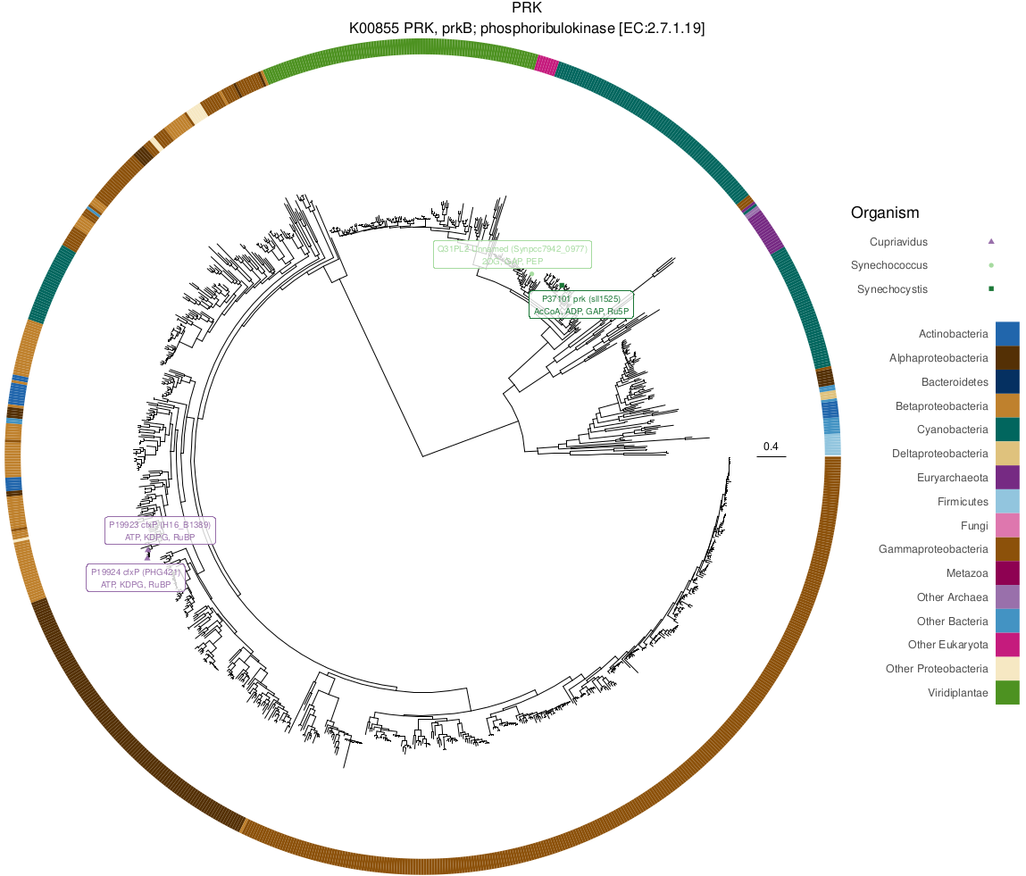
Phylogenetic trees of Calvin cycle genes were plotted using phytools and ggtree in R:
Rscript source/phylogenetics.R ${INFILE} ${OUTDIR}/phylogenetics
...producing the following final PDF containing visualizations of all trees, highlighting interactions with metabolites (Fig 4):
cbb_ko_trees.pdf
 |
|---|
| Fig 4. PRK phylogenetic tree with LiP-SMap interactions. |
KEGG EC and module annotations were combined with eggNOG orthologs and categories to give context to metabolite-protein interactions for low and high concentration:
Rscript source/tables.R ${INFILE} ${OUTDIR}/tables
...yielding a long format supplementary table:
ortholog_ec_module_interactions.xlsx
Calvin (CBB) cycle enzymes and related sink (or "drain") enzymes were investigated for interactions with the tested metabolites:
Rscript source/cbb.R ${INFILE} ${OUTDIR}/cbb
...by creating a plot of all interactions:
cbb.pdf
...with enzymes defined by EC number annotations from KEGG in the files data/cbb_enzymes.tab and data/cbb_drains.tab.
Carbon concentration mechanism (CCM) interactions in Synechocystis were plotted using this script:
Rscript source/ccm.R ${INFILE} ${OUTDIR}/ccm
...generating this output:
ccm.pdf
...based on CCM and regulatory genes listed in data/CCM_regulatory_proteins.csv.
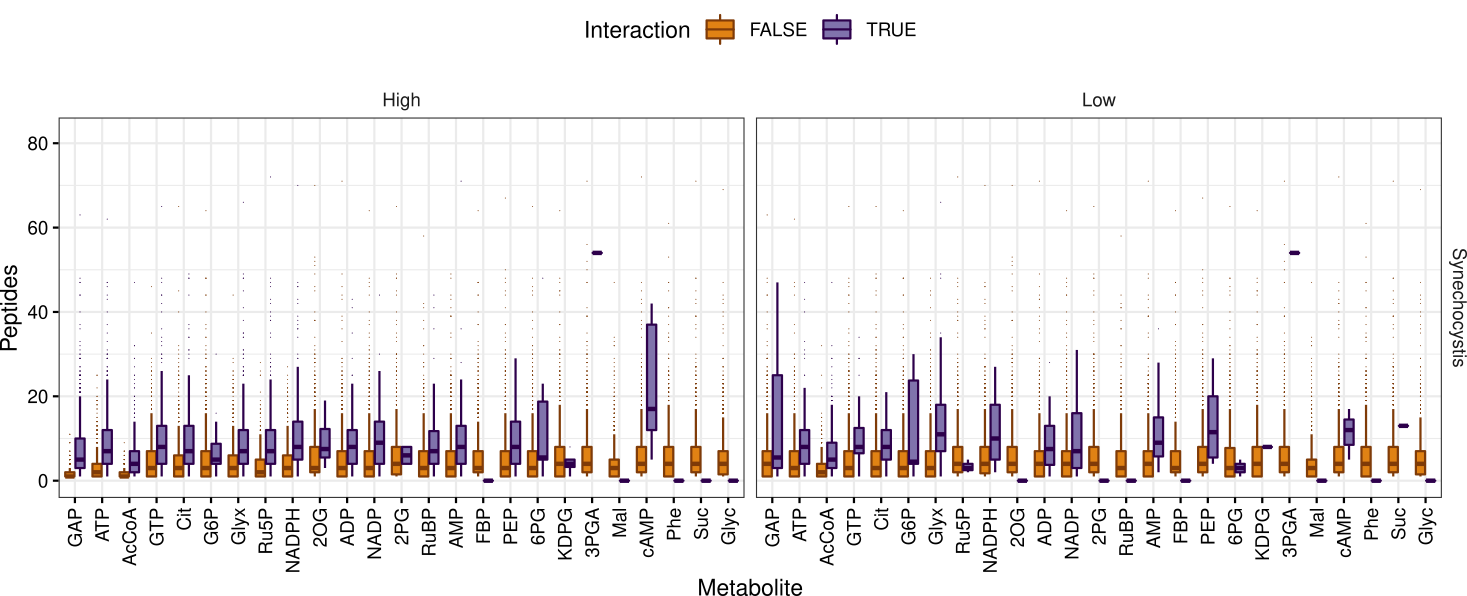
The number of detected peptides for proteins where none (Interaction FALSE) or at least one peptide (Interaction TRUE) showed significant interaction with a metabolite was plotted for each organism and concentration:
Rscript source/peptides.R ${INFILE} ${OUTDIR}/peptides
...yielding this graphic (Fig 5):
peptides_per_protein.pdf
Furthermore, the script counted the number of detected peptides in each experiment:
peptides_per_experiment.pdf
 |
|---|
| Fig 5. Detected peptides per protein compared to occurrence of interaction in Synechocystis. |
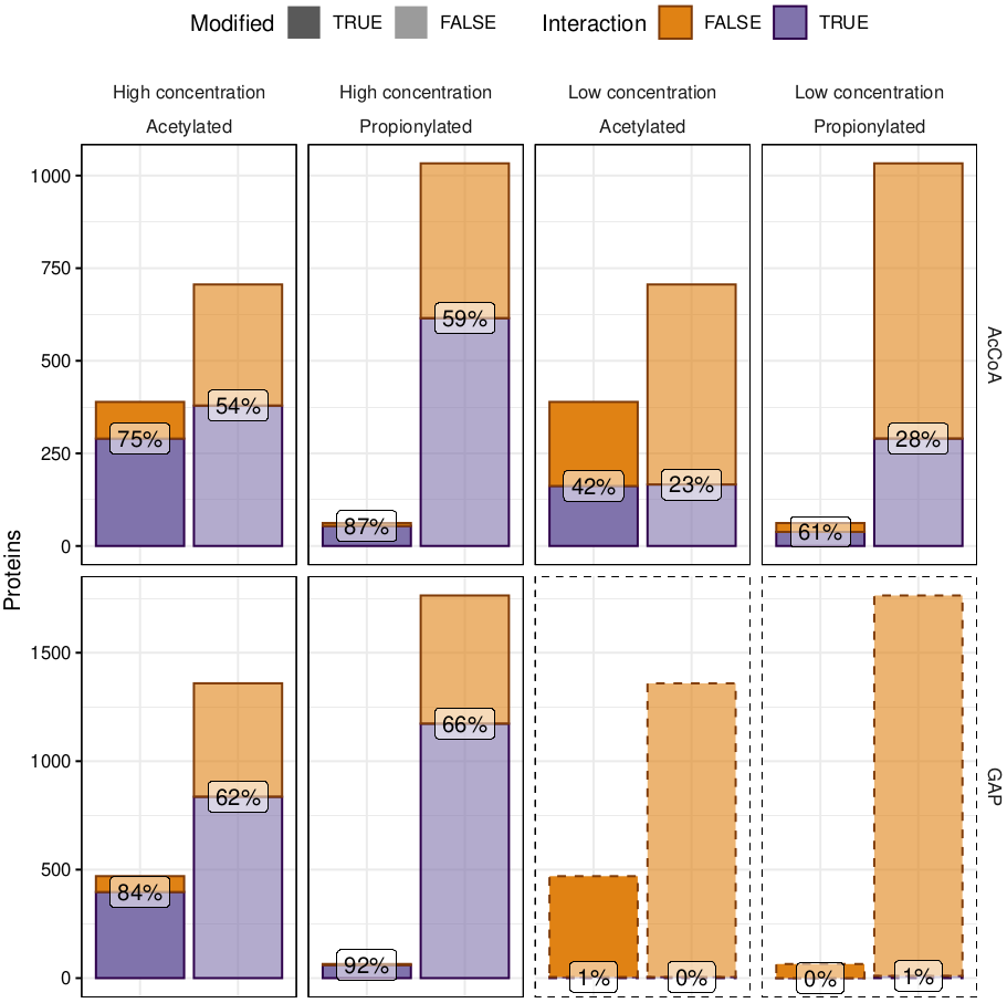
Interactions between Synechocystis proteins and acetyl-CoA or GAP were compared to published acetylome and propionylome data using Fisher's exact test followed by plotting:
Rscript source/modifications.R ${INFILE} ${OUTDIR}/modifications
...with this plot as the result (Fig 6):
modifications.pdf
 |
|---|
| Fig 6. Overlap between post-translational modifications and interactions with acetyl-CoA or GAP in Synechocystis (dashed lines indicate insignificant enrichment). |
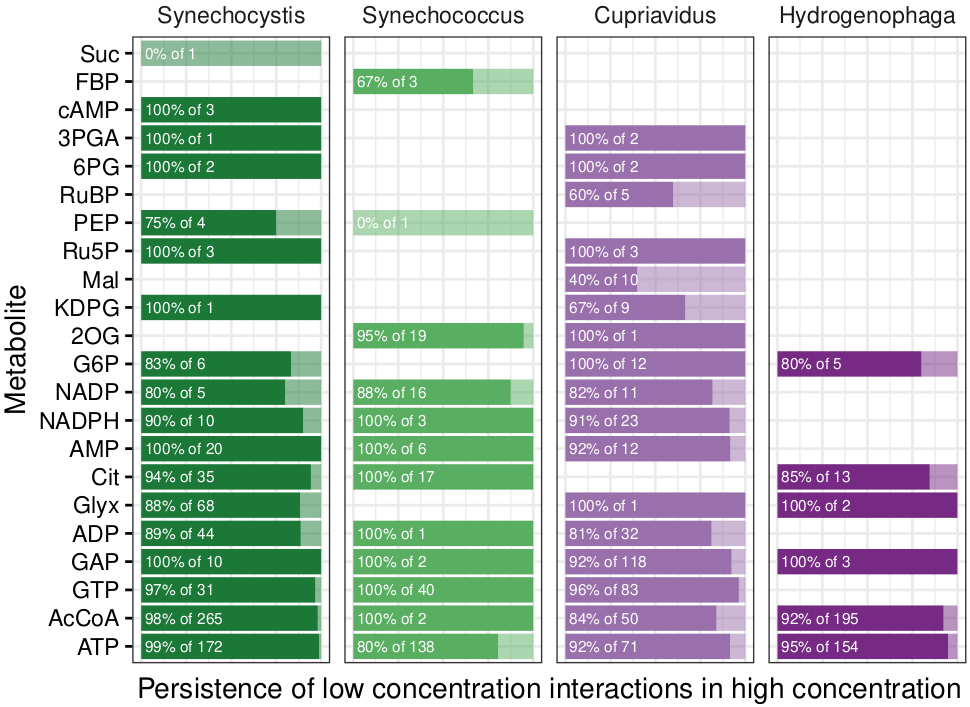
Quality of the experiments was assessed by checking persistence of significant low concentration interactions in high concentration (Fig 7), as well as correlating peptide fold changes in low and high concentration:
Rscript source/qc.R ${INFILE} ${OUTDIR}/qc
...which resulted in the following visualizations:
persistence.pdf
fc_correlation.png
 |
|---|
| Fig 7. Fraction interactions that persist from low to high concentration. |
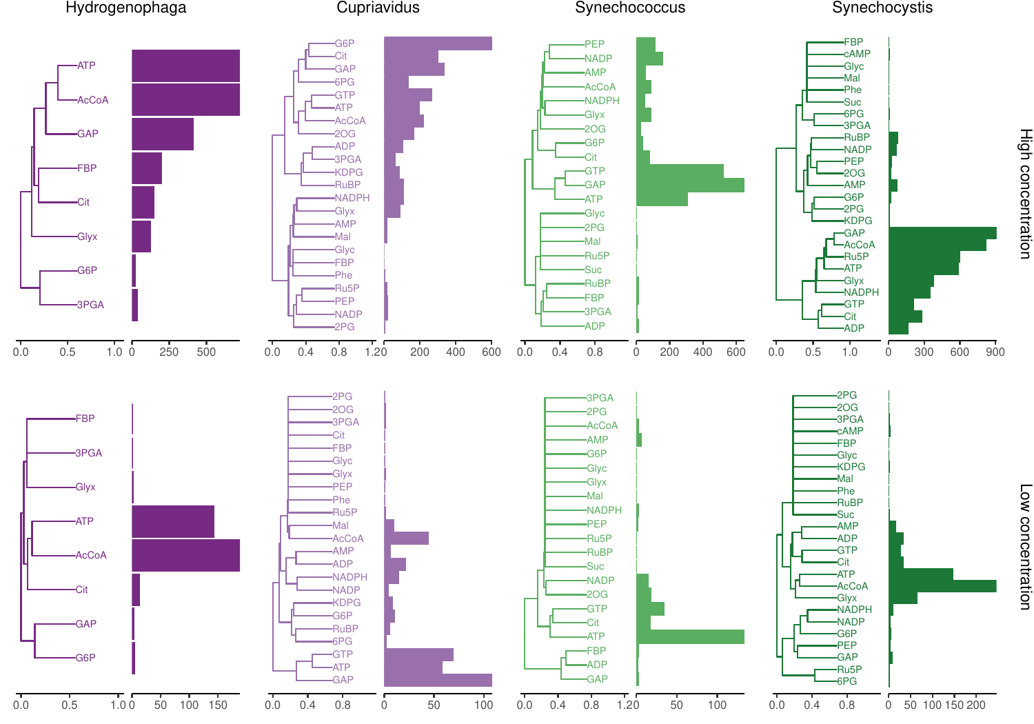
Metabolite-protein interaction patterns were compared within organisms with PCA and Jaccard distance/Ward.D2 hierarchical clustering using only proteins that were detected in all experiments. This is different from the ortholog interactions clustering since it is based on all detected proteins in each organism and not only orthologs found in all organisms. The analysis in this step was invoked as such:
Rscript source/metabolites.R ${INFILE} ${OUTDIR}/metabolites
...and yielded a PCA plot and a hierarchical clustering plot (Fig 8):
metabolites_pca.pdf
metabolites_jaccard_ward_D2.pdf
 |
|---|
| Fig 8. Clustering of metabolite-protein interaction patterns. Bars show number of proteins interacting with each metabolite. |
This tutorial demonstrates how to concatenate data from the original source structure and then run all analysis scripts on those data. The example data used here are a subset of the full dataset containing fewer metabolites and a random subset of 250 proteins per organism. It is therefore not representative of the full dataset.
Important: Before starting, make sure that the requirements are met. For running only the tutorial or the analysis pipeline it is enough to meet the R, Bash, and GNU parallel requirements.
The lipsmap repository should be installed on the target computer like so:
git clone https://github.com/Asplund-Samuelsson/lipsmap
The installation takes approximately five seconds, depending on the speed of the internet connection. After it finishes, change directory into the lipsmap repository:
cd lipsmap
The first step is to concatenate the input data from multiple LiP-SMap experiments in different organisms. Note that the pipeline described in this repository is specifically written to accommodate Hydrogenophaga, Cupriavidus, Synechococcus, and Synechocystis, and would require modification to accept other organisms.
The input data comes in multiple files:
data/tutorial/lipsmap/Cupriavidus/comparisonResult_3PGA_7_grouped_annot_20200914.csv
...
data/tutorial/lipsmap/Cupriavidus/comparisonResult_RuBP_7_grouped_annot_20200914.csv

data/tutorial/lipsmap/Hydrogenophaga/comparisonResult_3PGA_16_grouped_annot_20210527.csv
...
data/tutorial/lipsmap/Hydrogenophaga/comparisonResult_Glyx_17_grouped_annot_20210603.csv

data/tutorial/lipsmap/Synechococcus/comparisonResult_3PGA_13_grouped_annot_20210219.csv
...
data/tutorial/lipsmap/Synechococcus/comparisonResult_RuBP_14_grouped_annot_20210329.csv

data/tutorial/lipsmap/Synechocystis/comparisonResult_3PGA_13_grouped_annot_20210219.csv
...
data/tutorial/lipsmap/Synechocystis/comparisonResult_RuBP_11_grouped_annot_20210113.csv
We concatenate the files and make some corrections to locus IDs with an R script:
Rscript source/concatenate_input_data.R data/tutorial/lipsmap data/tutorial/lipsmap.tab.gz
Thereby we get the following compressed data file to be used with the analysis pipeline:
data/tutorial/lipsmap.tab.gz
Important: The concatenated data contains only the latest experiment, as defined by the date in the file names. If an earlier experiment is desired, one must remove the more recent file from the input directory. Another option is to set up a new input directory and populate it with symbolic links to the desired input files.
The analysis pipeline consists of many independent steps carried out by individual R scripts stored in the source directory. For convenience, a Bash script is set up to run all the steps automatically from a single command:
./analysis.sh data/tutorial/lipsmap.tab.gz results/tutorial
The pipeline finishes in less than two minutes, depending on the performance of the computer.
Messages from the individual pipeline scripts, for example errors, are stored in a log file:
results/tutorial/analysis.log
The analysis pipeline stores the results in one subdirectory per script:
results/tutorial/cbb/
results/tutorial/ccm/
results/tutorial/enzymes/
results/tutorial/functions/
results/tutorial/metabolites/
results/tutorial/modifications/
results/tutorial/modules/
results/tutorial/orthologs/
results/tutorial/peptides/
results/tutorial/phylogenetics/
results/tutorial/qc/
results/tutorial/tables/
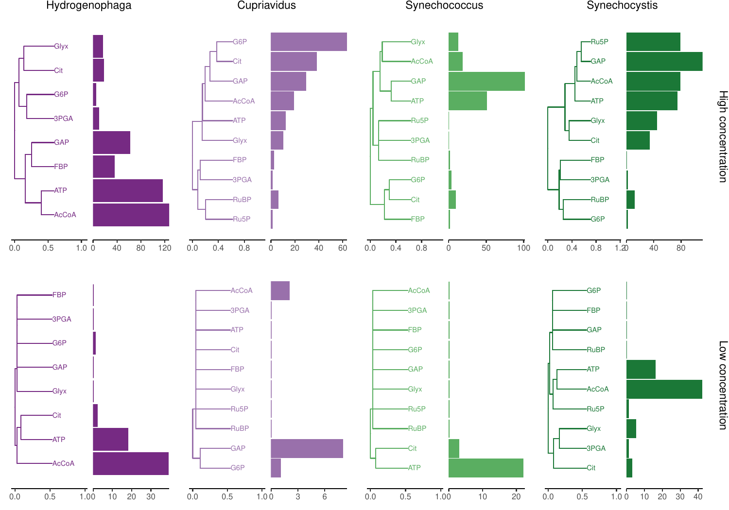
The tutorial output is available in this repository to demonstrate what it should look like. One example is to compare the hierarchical clustering of a complete dataset (Fig 8) and the reduced tutorial dataset (Fig 9).
 |
|---|
| Fig 9. Clustering of metabolite-protein interaction patterns in the tutorial dataset. Bars show number of proteins interacting with each metabolite. |
This analysis has been tested on a 12-core 32 GB RAM Linux system with Ubuntu 20.04 LTS and the following software:
| Program | Version | Libraries | |
|---|---|---|---|
| Bash | 5.0.17 | * | |
| R | 4.1.1 | ape, doMC, foreach, ggpubr, ggrepel, ggtree, openxlsx, phytools, scales, tidyverse, vegan | * |
| Python | 3.7.6 | Biopython | |
| CD-HIT | 4.8.1 | ||
| seqmagick | 0.8.0 | ||
| MAFFT | 7.453 | ||
| FastTree | 2.1.11 | ||
| GNU parallel | 20161222 | * |
*Required for concatenating data and running the analysis pipeline.
Johannes Asplund-Samuelsson ([email protected])
