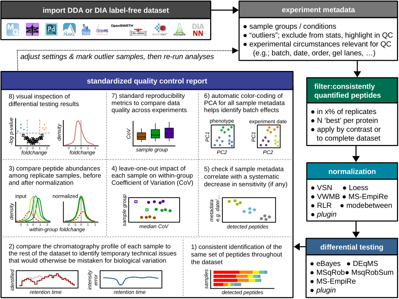
The Mass Spectrometry Downstream Analysis Pipeline is an all-in-one tool for the interpretation of label-free proteomics datasets. Its main features are extensive quality control, integration of state-of-the-art algorithms for differential testing and intuitive visualization and reporting. A novel algorithm for data normalization between experimental conditions is also included.
We are currently preparing a manuscript for publication, feel free to explore the documentation and test the beta-version of MS-DAP in this GitHub repository meanwhile !
Check this introduction to MS-DAP for an overview of data visualizations (example PDF reports are available at this link, bottom of the page).
Installation of the R package in brief, assuming R, RTools (v3.5 for R 3.6, v4 for R 4.0 and up) and RStudio have been installed (documentation references @ next section)
install.packages(c("devtools", "tidyverse", "tinytex", "BiocManager"))
tinytex::install_tinytex()
# On Windows; say 'no' to optionally compile packages and during TinyTex installation you may see 2 popups; these can be dismissed
BiocManager::install(c('ProtGenerics', 'MSnbase', 'limma'), update=T, ask=F)
Sys.setenv(R_REMOTES_NO_ERRORS_FROM_WARNINGS="true")
devtools::install_github("ftwkoopmans/msdap", upgrade = "never") # don't update dependencies if not needed
Example for analyzing a DIA dataset processed by DIA-NN (check the user guide for replacing DIA-NN input with Spectronaut, MaxQuant, etc.)
library(msdap)
# set the working directory to the full path where your data is stored (optionally, skip and use full paths below)
# importantly, use forward slashes for the path (so not "C:\temp" but "C:/temp")
setwd("C:/path/to/myproject")                                           # <<EDIT THIS FILENAME>>

# 1) Load data files, output from upstream raw data processor and the exact same fasta file(s) used there
dataset = import_dataset_diann(filename = "diann_resulting_report.tsv") # <<EDIT THIS FILENAME>>
dataset = import_fasta(dataset, files = "proteome.fasta")               # <<EDIT THIS FILENAME>>

# 2) Create a template file that describes all samples. A new Excel table will be created at this path
# - note; you only have to do steps 2 and 3 once per dataset
write_template_for_sample_metadata(dataset, "sample_metadata.xlsx")

# 3) Time to step away from R for a sec, and edit this template file in Excel or LibreOffice;
# - describe the sample group of each sample in the "group" column
# - add additional columns with any metadata that varies between samples (measurement order, gel, gel lane, batch, etc.) -->> QC figures will be auto generated
# - further documentation is available in the "instructions" tab within the Excel file

# 4) Load sample metadata from file you just edited (don't forget to save it first)
dataset = import_sample_metadata(dataset, filename = "sample_metadata.xlsx")

# 5) Optionally, describe a statistical contrast; in this example we compare sample groups "WT" and "KO".
# - You should use exact same labels as "group" column in sample metadata table.
# - If you don't want to do stats, simply remove or comment this line (e.g. just look at QC report, or maybe your dataset has 1 experimental group only).
# - example for multiple contrasts; dataset = setup_contrasts(dataset, contrast_list = list( c("control", "condition_a"),  c("control", "condition_b")  ) )
# - example for adding random variables to eBayes/DEqMS/MSqRob regressions to i.e. counter batch effects (note; these variables must be column names present in sample metadata table. double-check with; print(dataset$samples,n=Inf)): dataset = setup_contrasts(dataset, contrast_list = list(  c("WT","KO")  ), random_variables = c("induction", "batch") )
dataset = setup_contrasts(dataset, contrast_list = list(  c("WT","KO")  ) )

# 6) Main function that runs the entire pipeline
# for DIA, recommended settings are defined below, selecting only peptides that were confidently detected in most samples
# for DDA, 'confident detection' relies on MS/MS which may be more rare (relying on match-between-runs instead)
# following benchmarks in the MS-DAP manuscript, for DDA we recommend to set no or minimal requirements on 'detect' parameters; "filter_fraction_detect = 0" and "filter_min_detect = 0" (or 1 if you want at least 1 MS/MS detect per peptide per sample group)
dataset = analysis_quickstart(
  dataset,
  filter_min_detect = 3,         # each peptide must have a good confidence score in at least N samples per group
  filter_min_quant = 3,          # similarly, the number of reps where the peptide must have a quantitative value
  filter_fraction_detect = 0.75, # each peptide must have a good confidence score in at least 75% of samples per group
  filter_fraction_quant = 0.75,  # analogous for quantitative values
  filter_by_contrast = TRUE,     # only relevant if dataset has 3+ groups. For DEA at each contrast, filters and normalization are applied on the subset of relevant samples within the contrast for efficiency, see further MS-DAP manuscript. Set to FALSE to disable and use traditional "global filtering" (filters are applied to all sample groups, same data table used in all statistics)
  norm_algorithm = c("vsn", "modebetween_protein"), # normalization; first vsn, then modebetween on protein-level (applied sequentially so the MS-DAP modebetween algorithm corrects scaling/balance between-sample-groups)
  dea_algorithm = c("deqms", "msempire", "msqrob"), # statistics; apply multiple methods in parallel/independently
  dea_qvalue_threshold = 0.01,                      # threshold for significance of adjusted p-values in figures and output tables
  dea_log2foldchange_threshold = NA,                # threshold for significance of log2 foldchanges. 0 = disable, NA = automatically infer through bootstrapping
  output_qc_report = TRUE,                          # optionally, set to FALSE to skip the creation of the QC report (not recommended for first-time use)
  output_abundance_tables = TRUE,                   # optionally, disable the creation of abundance table output files
  output_dir = "msdap_results",                    # output directory, here set to "msdap_results" within your working directory. Alternatively provide a full path, eg; output_dir="C:/path/to/myproject",
  output_within_timestamped_subdirectory = TRUE )
# print a short summary of results at the end
print_dataset_summary(dataset)

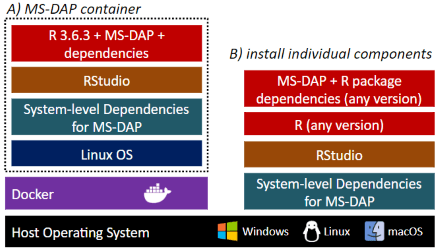
# 7) All done! Check out the generated files in the output directory, starting with report.pdfMS-DAP is available as a Docker container that includes everything required to get starting right away, and as a R package that may be installed into a preexisting bioinformatics workflow.
-
Installing the dockerized version of MS-DAP is trivialized to first installing the Docker application and then pulling the MS-DAP container from the online Docker repository ( as shown in this guide ). Using containers guarantees the exact same software versions are used throughout the entire stack, from operating system to the actual application, a crucial aspect of software reproducibility. As the MS-DAP application matures, users can re-run analyses on any legacy MS-DAP release by simply pulling the respective container version (e.g. to repeat a previously published analysis).
-
Already working with R? Click here for an installation guide to install the MS-DAP R package.
The introduction vignette illustrates how MS-DAP works and showcases a diverse set of data visualizations from real datasets to highlight how MS-DAP can help you extract more value from your experimental data.
The second vignette is a more hands-on tutorial that describes how to prepare input data and how to configure parameters of this data analysis pipeline.
Bioinformatic analyses beyond the typical MS-DAP workflow are described in the following vignettes, from a more detailed look at differential testing to integrating alternative algorithms for normalization or Differential Expression Analysis (DEA).
- introduction to MS-DAP
- user guide
- bioinformatics: differential expression analysis (DEA)
- bioinformatics: differential detection
- bioinformatics: plugin custom normalization or DEA
Features planned for future releases:
- expand upstream software support
- labeled quantitative data; iTRAQ/TMT


