🏡💰🏡💰🏡

This project was an attempt to the iNeuron ML Challenge 2. The main objective of the project was to predict monthly house rent depending upon the various features.
The data set could be found on the iNeuron challenge website linked above.
The dataset contains 265190 records of house, a huge number of these records are mostly from the United States with few outliers. The dataset has 22 features, features including various urls, the price, the sqfeet, numeber of beds and baths, description, region etc.
Here is a map showing the house records. As we can see most of the houses are from the United States.

Let's look at the statistical description of our data
| Desc | price | sqfeet | beds | baths | lat | long |
|---|---|---|---|---|---|---|
| count | 2.651900e+05 | 2.651900e+05 | 265190.000000 | 265190.000000 | 263771.000000 | 263771.000000 |
| mean | 1.227285e+04 | 1.093678e+03 | 1.912414 | 1.483468 | 37.208855 | -92.398149 |
| std | 5.376352e+06 | 2.306888e+04 | 3.691900 | 0.630208 | 5.659648 | 17.370780 |
| min | 0.000000e+00 | 0.000000e+00 | 0.000000 | 0.000000 | -43.533300 | -163.894000 |
| 25% | 8.170000e+02 | 7.520000e+02 | 1.000000 | 1.000000 | 33.508500 | -104.704000 |
| 50% | 1.060000e+03 | 9.500000e+02 | 2.000000 | 1.000000 | 37.984900 | -86.478300 |
| 75% | 1.450000e+03 | 1.156000e+03 | 2.000000 | 2.000000 | 41.168400 | -81.284600 |
| max | 2.768307e+09 | 8.388607e+06 | 1100.000000 | 75.000000 | 102.036000 | 172.633000 |
The target variable, here price was highly skewed towards the left side with skewness of 514.78 and kurtosis of 265062.43

The skewness of the data points are resolved after log transformation. Log transformation gave us a skewness of 4.47 and kurtosis of 52.47

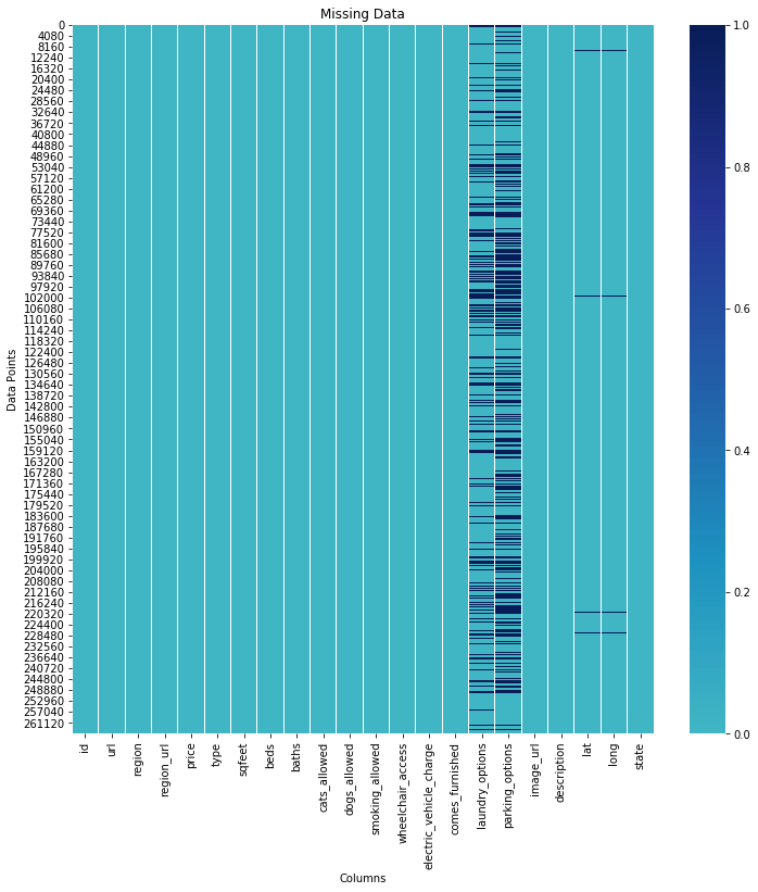
The features containing missing values are:
- parking_options (36%)
- laundry_options (20%)
- lat (0.5%)
- long (0.5%)
- description & state (nominal percentage)

Imputate missing values Here's my take on imputing these missing values:
| variables | imputation |
|---|---|
| parking_options | mode value of the parking_options for the respective house type |
| laundry_options | mode value of the laundry_options for the respective house type |
| lat | mode value of the lattitude for the respective house region |
| long | mode value of the longitude for the respective house region |
| state | drop records |
| description | drop records |
Percentage description of the various house types in our dataset

As we can see apartment acquires around 50% of our dataset, followed by house(7.07%) and flat(5.87%)

As we can see, there is no strong correlation among the independent variables with the dependent variables. Therefore, a linear model will perform terribly in this dataset.
While going through the description of few house records, I came across some interesting information as in houses having a pool, a gym nearby, a fireplace or a shopping mall nearby. I think this information will make a few good features. So I went ahead and made these new features.
Also, as our data was not normally distribute. Performed log transformation on numerical data.
And saved the cleaned dataset to a csv.
4 different learning regressors (Linear Regression, Random Forest, Gradient Boosting, and XgBoost) were tested, and we have achieved the best prediction performance using Random Forest, followed by Gradient Boosting, then XgBoost, while Linear Regression achieved the worst performance of the four.
The best prediction performance was achieved with a Random Forest regressor, using all features in the dataset, and resulted in the following metrics:
- Mean Absolute Error (MAE): 0.059128200788923446
- Root mean squared error (RMSE): 0.1717131883398518
- R-squared Score (R2_Score): 0.8746976791953469


- A Simple Tutorial To Data Visualization: Kaggle notebook by Vansh Jatana
- Outlier Detection Techniques: Simplified: Kaggle notebook by Suraj RP
- Towards Data Science blog: Easy Steps To Plot Geographic Data on a Map — Python
- Plotly documentation: https://plotly.com/python/
- Folium documentation: https://python-visualization.github.io/folium/quickstart.html