Project idea inspired from Samson Zhang. Design and implementation are quite different from the one in his Kaggle Notebook that

• This implementation uses Numba to speed up the computations
• Uses OOP to modularize code.
• Uses the real MNIST Idx data sets, instead of the Kaggle provided .csv files.
• Includes separate classes for handling Idx1, Idx3 IO.
• NNetworkMinimal class can save a trained model's state to disk and reconstruct the trained model from the serialized model file. This prevents the need to retrain the model from scratch to make predictions again, granted that the training dataset hasn't been altered since the last training.

MNIST

Outline of the NNetworkMinimal class training process

• The NNetworkMinimal class represents a very simple fully connected three layer neural network. The input layer has 784 neurons, each designated to handle one pixel from the training image.
• The middle (aka hidden) layer has 10 neurons, fully connected to the input and output layers.
• The output layer has 10 neurons, each registering the probability of the given image representing the n th digit (the digits (predictions) can be 0 through 9, hence the 10 neurons).
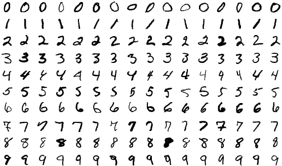
• The training images are arrays of 28 x 28 black and white pixels (each one byte in size, with 0 mapping to black and 255 mapping to white).
• The training happens in batches, so instead of processing each image (i.e an array of 28 x 28 pixels), we'll treat the N number of images as a matrix which embodies 28 x 28 rows and N columns.
• In other words, in lieu of iteratively passing every image through all the layers (in both forward and backward propagations) we'll be passing arrays of images.
• Here, the rows represent a select pixel from all the N images and a column holds all the 28 x 28 pixels of an image.

The matrix can also be reimagined as a tensor with (28, 28, N) dimensions

$I_{[784, ~N]} \Longrightarrow H_{[10, ~N]} \Longrightarrow O_{[10, ~N]}$

A matrix notation $M_{[r,~c]}$ indicates a matrix with r rows and c columns, not the matrix element at r th row and c th column!.

Forward propagation

$H_{[10, ~N]} = W_{[784, ~10]} \cdot I_{[784, ~N]} + B_{[10, ~1]}$

${\hat{H}}_{[10, ~N]} = {f(H_{[10, ~N]})}$

${\hat{H}}_{[10, N]} = {ReLU(H)}_{[10, N]}$

$ReLU(x): ~ x ~ if ~ (x > 0) ~ else ~ 0$

${O}_{[10, N]} = {w}_{[10, 10]} \cdot {\hat{H}}_{[10, N]} + {b}_{[10, 1]}$

${\hat{O}}_{[10, N]} = {f_{softmax}(O)}_{[10, N]}$

$softmax = \frac{e^O}{\sum_{j = 1}^{K} e_{j}^O}$

$softmax = ({\begin{bmatrix} 0.9 \\ 1.7 \\ 8.4 \\ \vdots \\ 2.1 \\ 8.5 \\ 9.1 \\ \end{bmatrix}})_{[10, 1]}$

{\begin{bmatrix} 0.10 \ 0.23 \ 0.00 \ \vdots \ 0.74 \ 0.01 \ 0.01 \ \end{bmatrix}}_{10, 1}$

Phase 2) Back propagation

prediction = {\begin{bmatrix} 0.01 \ 0.05 \ 0.69 \ \vdots \ 0.00 \ 0.10 \ 0.07 \ \end{bmatrix}}_{10, 1} \

\text{one hot encoded label} = {\begin{bmatrix} 0 \ 0 \ 1 \ \vdots \ 0 \ 0 \ 0 \ \end{bmatrix}}_{10, 1} \

{\mathrm{d}O}{10, N} = {\hat{O}}{10, N} - {L_{True}}_{10, N} \

\mathrm{d}O_i = \begin{bmatrix} 0.01 \ 0.05 \ 0.69 \ \vdots \ 0.00 \ 0.10 \ 0.07 \ \end{bmatrix} - \begin{bmatrix} 0 \ 0 \ 1 \ \vdots \ 0 \ 0 \ 0 \ \end{bmatrix} \

{\mathrm{d}{w}}_{10, 10} = \frac{ \overbrace{\mathrm{d}{O}}^{10, N} \cdot \overbrace{\hat{H}^T}^{N, 10}}{N} \

{\mathrm{d}{b}}{10, 1} = \frac{\sum{i~=~1}^{N}{\overbrace{\mathrm{d}{O_i}}^{10, 1}}}{N} \

{\mathrm{d}{H}}{10, N} = {w^T}{10, 10} \cdot {\mathrm{d}{O}}{10, N}, {f^{\prime}(H)}{10, N} \

{\mathrm{d}{W}}_{10, 784} = \frac{\overbrace{\mathrm{d}{H}}^{10, N} \cdot \overbrace{I^T}^{N, 784}}{N} \

{\mathrm{d}{B}}{10, 1} = \frac{\sum{i~=~1}^{N}{\overbrace{\mathrm{d}{H_i}}^{10, 1}}}{N} \

Phase 3) Simultaneous paramater updates

W = W - $\alpha$ dW
B = B - $\alpha$ dB
w = w - $\alpha$ dw
b = b - $\alpha$ db

$\alpha$ - learning rate

After 5,000 iterations, the accuracy scores for MNIST datasets were:

• Training dataset - 0.935367 (93.54%)
• Test dataset - 0.928800 (92.88%)

For a thorough, step by step walkthrough, refer the source code. It's comprehensively annotated!

Fashion MNIST

Using the same NNetworkMinimal class used for MNIST datasets with 5000 iterations, the accuracy scores for Fashion MNIST datasets were:

• Training dataset - 0.262367 (26.24%)
• Test dataset - 0.263800 (26.38%)

Fashion MNIST datasets was designed intentionally as a superior alternative to the MNIST datasets as the former is too simple that even a naive network could make decent predictions using it. The problem with MNIST is that the information encoded in the image pixels are not that complex to easily materialize a good enough digit classifier.

As Fashion MNIST introduces more sophisticated visually similar shapes, the model now needs to capture more nuanced, granular patterns in the images to make good enough predictions (e.g. the visual differences between a woman's top and a tshirt aren't as pronounced as the differences between the digits 1 and 2, particularly in low resolution images (28 x 28 pixels to be precise)). Our NNetworkMinimal class design is way too simple for complex learning endeavours, hence the poor accuracy scores with Fashion MNIST datasets.

This is the rationale for the NNExtended subproject, to implement a model sophisticated enough to make decent predictions on Fashion MNIST datasets, but this time in C++.