forked from mitmath/matrixcalc
-
Notifications
You must be signed in to change notification settings - Fork 0
/
automatic_differentiation_done_quick.jmd
1043 lines (754 loc) · 38.8 KB
/
automatic_differentiation_done_quick.jmd
1
2
3
4
5
6
7
8
9
10
11
12
13
14
15
16
17
18
19
20
21
22
23
24
25
26
27
28
29
30
31
32
33
34
35
36
37
38
39
40
41
42
43
44
45
46
47
48
49
50
51
52
53
54
55
56
57
58
59
60
61
62
63
64
65
66
67
68
69
70
71
72
73
74
75
76
77
78
79
80
81
82
83
84
85
86
87
88
89
90
91
92
93
94
95
96
97
98
99
100
101
102
103
104
105
106
107
108
109
110
111
112
113
114
115
116
117
118
119
120
121
122
123
124
125
126
127
128
129
130
131
132
133
134
135
136
137
138
139
140
141
142
143
144
145
146
147
148
149
150
151
152
153
154
155
156
157
158
159
160
161
162
163
164
165
166
167
168
169
170
171
172
173
174
175
176
177
178
179
180
181
182
183
184
185
186
187
188
189
190
191
192
193
194
195
196
197
198
199
200
201
202
203
204
205
206
207
208
209
210
211
212
213
214
215
216
217
218
219
220
221
222
223
224
225
226
227
228
229
230
231
232
233
234
235
236
237
238
239
240
241
242
243
244
245
246
247
248
249
250
251
252
253
254
255
256
257
258
259
260
261
262
263
264
265
266
267
268
269
270
271
272
273
274
275
276
277
278
279
280
281
282
283
284
285
286
287
288
289
290
291
292
293
294
295
296
297
298
299
300
301
302
303
304
305
306
307
308
309
310
311
312
313
314
315
316
317
318
319
320
321
322
323
324
325
326
327
328
329
330
331
332
333
334
335
336
337
338
339
340
341
342
343
344
345
346
347
348
349
350
351
352
353
354
355
356
357
358
359
360
361
362
363
364
365
366
367
368
369
370
371
372
373
374
375
376
377
378
379
380
381
382
383
384
385
386
387
388
389
390
391
392
393
394
395
396
397
398
399
400
401
402
403
404
405
406
407
408
409
410
411
412
413
414
415
416
417
418
419
420
421
422
423
424
425
426
427
428
429
430
431
432
433
434
435
436
437
438
439
440
441
442
443
444
445
446
447
448
449
450
451
452
453
454
455
456
457
458
459
460
461
462
463
464
465
466
467
468
469
470
471
472
473
474
475
476
477
478
479
480
481
482
483
484
485
486
487
488
489
490
491
492
493
494
495
496
497
498
499
500
501
502
503
504
505
506
507
508
509
510
511
512
513
514
515
516
517
518
519
520
521
522
523
524
525
526
527
528
529
530
531
532
533
534
535
536
537
538
539
540
541
542
543
544
545
546
547
548
549
550
551
552
553
554
555
556
557
558
559
560
561
562
563
564
565
566
567
568
569
570
571
572
573
574
575
576
577
578
579
580
581
582
583
584
585
586
587
588
589
590
591
592
593
594
595
596
597
598
599
600
601
602
603
604
605
606
607
608
609
610
611
612
613
614
615
616
617
618
619
620
621
622
623
624
625
626
627
628
629
630
631
632
633
634
635
636
637
638
639
640
641
642
643
644
645
646
647
648
649
650
651
652
653
654
655
656
657
658
659
660
661
662
663
664
665
666
667
668
669
670
671
672
673
674
675
676
677
678
679
680
681
682
683
684
685
686
687
688
689
690
691
692
693
694
695
696
697
698
699
700
701
702
703
704
705
706
707
708
709
710
711
712
713
714
715
716
717
718
719
720
721
722
723
724
725
726
727
728
729
730
731
732
733
734
735
736
737
738
739
740
741
742
743
744
745
746
747
748
749
750
751
752
753
754
755
756
757
758
759
760
761
762
763
764
765
766
767
768
769
770
771
772
773
774
775
776
777
778
779
780
781
782
783
784
785
786
787
788
789
790
791
792
793
794
795
796
797
798
799
800
801
802
803
804
805
806
807
808
809
810
811
812
813
814
815
816
817
818
819
820
821
822
823
824
825
826
827
828
829
830
831
832
833
834
835
836
837
838
839
840
841
842
843
844
845
846
847
848
849
850
851
852
853
854
855
856
857
858
859
860
861
862
863
864
865
866
867
868
869
870
871
872
873
874
875
876
877
878
879
880
881
882
883
884
885
886
887
888
889
890
891
892
893
894
895
896
897
898
899
900
901
902
903
904
905
906
907
908
909
910
911
912
913
914
915
916
917
918
919
920
921
922
923
924
925
926
927
928
929
930
931
932
933
934
935
936
937
938
939
940
941
942
943
944
945
946
947
948
949
950
951
952
953
954
955
956
957
958
959
960
961
962
963
964
965
966
967
968
969
970
971
972
973
974
975
976
977
978
979
980
981
982
983
984
985
986
987
988
989
990
991
992
993
994
995
996
997
998
999
1000
---
title: Forward and Reverse Automatic Differentiation In A Nutshell
author: Chris Rackauckas
date: January 21st, 2022
---
# Machine Epsilon and Roundoff Error
Floating point arithmetic is relatively scaled, which means that the precision
that you get from calculations is relative to the size of the floating point
numbers. Generally, you have 16 digits of accuracy in (64-bit) floating
point operations. To measure this, we define *machine epsilon* as the value
by which `1 + E = 1`. For floating point numbers, this is:
```julia
eps(Float64)
```
However, since it's relative, this value changes as we change our reference value:
```julia
@show eps(1.0)
@show eps(0.1)
@show eps(0.01)
```
Thus issues with *roundoff error* come when one subtracts out the higher digits.
For example, $(x + \epsilon) - x$ should just be $\epsilon$ if there was no
roundoff error, but if $\epsilon$ is small then this kicks in. If $x = 1$
and $\epsilon$ is of size around $10^{-10}$, then $x+ \epsilon$ is correct for
10 digits, dropping off the smallest 6 due to error in the addition to $1$.
But when you subtract off $x$, you don't get those digits back, and thus you
only have 6 digits of $\epsilon$ correct.
Let's see this in action:
```julia
ϵ = 1e-10rand()
@show ϵ
@show (1+ϵ)
ϵ2 = (1+ϵ) - 1
(ϵ - ϵ2)
```
See how $\epsilon$ is only rebuilt at accuracy around $10^{-16}$ and thus we only
keep around 6 digits of accuracy when it's generated at the size of around $10^{-10}$!
## Finite Differencing and Numerical Stability
To start understanding how to compute derivatives on a computer, we start with
*finite differencing*. For finite differencing, recall that the definition of
the derivative is:
$$f'(x) = \lim_{\epsilon \rightarrow 0} \frac{f(x+\epsilon)-f(x)}{\epsilon}$$
Finite differencing directly follows from this definition by choosing a small
$\epsilon$. However, choosing a good $\epsilon$ is very difficult. If $\epsilon$
is too large than there is error since this definition is asymtopic. However,
if $\epsilon$ is too small, you receive roundoff error. To understand why
you would get roundoff error, recall that floating point error is relative,
and can essentially store 16 digits of accuracy. So let's say we choose
$\epsilon = 10^{-6}$. Then $f(x+\epsilon) - f(x)$ is roughly the same in the
first 6 digits, meaning that after the subtraction there is only 10 digits of
accuracy, and then dividing by $10^{-6}$ simply brings those 10 digits back up
to the correct relative size.

This means that we want to choose $\epsilon$ small enough that the
$\mathcal{O}(\epsilon^2)$ error of the truncation is balanced by the $O(1/\epsilon)$
roundoff error. Under some minor assumptions, one can argue that the average
best point is $\sqrt(E)$, where E is machine epsilon
```julia
@show eps(Float64)
@show sqrt(eps(Float64))
```
This means we should not expect better than 8 digits of accuracy, even when
things are good with finite differencing.

The centered difference formula is a little bit better, but this picture
suggests something much better...
## Differencing in a Different Dimension: Complex Step Differentiation
The problem with finite differencing is that we are mixing our really small
number with the really large number, and so when we do the subtract we lose
accuracy. Instead, we want to keep the small perturbation completely separate.
To see how to do this, assume that $x \in \mathbb{R}$ and assume that $f$ is
complex analytic. You want to calculate a real derivative, but your function
just happens to also be complex analytic when extended to the complex plane.
Thus it has a Taylor series, and let's see what happens when we expand out this
Taylor series purely in the complex direction:
$$f(x+ih) = f(x) + f'(x)ih + \mathcal{O}(h^2)$$
which we can re-arrange as:
$$if'(x) = \frac{f(x+ih) - f(x)}{h} + \mathcal{O}(h)$$
Since $x$ is real and $f$ is real-valued on the reals, $if'$ is purely imaginary.
So let's take the imaginary parts of both sides:
$$f'(x) = \frac{Im(f(x+ih))}{h} + \mathcal{O}(h)$$
since $Im(f(x)) = 0$ (since it's real valued!). Thus with a sufficiently small
choice of $h$, this is the *complex step differentiation* formula for calculating
the derivative.
But to understand the computational advantage, recal that $x$ is pure real, and
thus $x+ih$ is an imaginary number where **the $h$ never directly interacts with
$x$** since a complex number is a two dimensional number where you keep the two
pieces separate. Thus there is no numerical cancellation by using a small value
of $h$, and thus, due to the relative precision of floating point numbers, both
the real and imaginary parts will be computed to (approximately) 16 digits of
accuracy for any choice of $h$.
## Derivatives as nilpotent sensitivities
The derivative measures the **sensitivity** of a function, i.e. how much the
function output changes when the input changes by a small amount $\epsilon$:
$$f(a + \epsilon) = f(a) + f'(a) \epsilon + o(\epsilon).$$
In the following we will ignore higher-order terms; formally we set
$\epsilon^2 = 0$. This form of analysis can be made rigorous through a form
of non-standard analysis called *Smooth Infinitesimal Analysis* [1], though
note that nilpotent infinitesimal requires *constructive logic*, and thus proof
by contradiction is not allowed in this logic due to a lack of the *law of the
excluded middle*.
A function $f$ will be represented by its value $f(a)$ and derivative $f'(a)$,
encoded as the coefficients of a degree-1 (Taylor) polynomial in $\epsilon$:
$$f \rightsquigarrow f(a) + \epsilon f'(a)$$
Conversely, if we have such an expansion in $\epsilon$ for a given function $f$,
then we can identify the coefficient of $\epsilon$ as the derivative of $f$.
## Dual numbers
Thus, to extend the idea of complex step differentiation beyond complex analytic
functions, we define a new number type, the *dual number*. A dual number is a
multidimensional number where the sensitivity of the function is propagated
along the dual portion.
Here we will now start to use $\epsilon$ as a dimensional signifier, like $i$,
$j$, or $k$ for quaternion numbers. In order for this to work out, we need
to derive an appropriate algebra for our numbers. To do this, we will look
at Taylor series to make our algebra reconstruct differentiation.
Note that the chain rule has been explicitly encoded in the derivative part.
$$f(a + \epsilon) = f(a) + \epsilon f'(a)$$
to first order. If we have two functions
$$f \rightsquigarrow f(a) + \epsilon f'(a)$$
$$g \rightsquigarrow g(a) + \epsilon g'(a)$$
then we can manipulate these Taylor expansions to calculate combinations of
these functions as follows. Using the nilpotent algebra, we have that:
$$(f + g) = [f(a) + g(a)] + \epsilon[f'(a) + g'(a)]$$
$$(f \cdot g) = [f(a) \cdot g(a)] + \epsilon[f(a) \cdot g'(a) + g(a) \cdot f'(a) ]$$
From these we can *infer* the derivatives by taking the component of $\epsilon$.
These also tell us the way to implement these in the computer.
## Computer representation
Setup (not necessary from the REPL):
```julia
using InteractiveUtils # only needed when using Weave
```
Each function requires two pieces of information and some particular "behavior",
so we store these in a `struct`. It's common to call this a "dual number":
```julia
struct Dual{T}
val::T # value
der::T # derivative
end
```
Each `Dual` object represents a function. We define arithmetic operations to
mirror performing those operations on the corresponding functions.
We must first import the operations from `Base`:
```julia
Base.:+(f::Dual, g::Dual) = Dual(f.val + g.val, f.der + g.der)
Base.:+(f::Dual, α::Number) = Dual(f.val + α, f.der)
Base.:+(α::Number, f::Dual) = f + α
#=
You can also write:
import Base: +
f::Dual + g::Dual = Dual(f.val + g.val, f.der + g.der)
=#
Base.:-(f::Dual, g::Dual) = Dual(f.val - g.val, f.der - g.der)
# Product Rule
Base.:*(f::Dual, g::Dual) = Dual(f.val*g.val, f.der*g.val + f.val*g.der)
Base.:*(α::Number, f::Dual) = Dual(f.val * α, f.der * α)
Base.:*(f::Dual, α::Number) = α * f
# Quotient Rule
Base.:/(f::Dual, g::Dual) = Dual(f.val/g.val, (f.der*g.val - f.val*g.der)/(g.val^2))
Base.:/(α::Number, f::Dual) = Dual(α/f.val, -α*f.der/f.val^2)
Base.:/(f::Dual, α::Number) = f * inv(α) # Dual(f.val/α, f.der * (1/α))
Base.:^(f::Dual, n::Integer) = Base.power_by_squaring(f, n) # use repeated squaring for integer powers
```
We can now define `Dual`s and manipulate them:
```julia
f = Dual(3, 4)
g = Dual(5, 6)
f + g
```
```julia
f * g
```
```julia
f * (g + g)
```
## Defining Higher Order Primitives
We can also define functions of `Dual` objects, using the chain rule.
To speed up our derivative function, we can directly hardcode the derivative
of known functions which we call *primitives*. If `f` is
a `Dual` representing the function $f$, then `exp(f)` should be a `Dual`
representing the function $\exp \circ f$, i.e. with value $\exp(f(a))$ and
derivative $(\exp \circ f)'(a) = \exp(f(a)) \, f'(a)$:
```julia
import Base: exp
```
```julia
exp(f::Dual) = Dual(exp(f.val), exp(f.val) * f.der)
```
```julia
f
```
```julia
exp(f)
```
# Differentiating arbitrary functions
For functions where we don't have a rule, we can recursively do dual number
arithmetic within the function until we hit primitives where we know the derivative,
and then use the chain rule to propagate the information back up.
Under this algebra, we can represent $a + \epsilon$ as `Dual(a, 1)`.
Thus, applying `f` to `Dual(a, 1)` should give `Dual(f(a), f'(a))`. This is thus
a 2-dimensional number for calculating the derivative without floating point
error, **using the compiler to transform our equations into dual number arithmetic**.
To to differentiate an arbitrary function, we define a generic function and then
change the algebra.
```julia
h(x) = x^2 + 2
a = 3
xx = Dual(a, 1)
```
Now we simply evaluate the function `h` at the `Dual` number `xx`:
```julia
h(xx)
```
The first component of the resulting `Dual` is the value $h(a)$, and the
second component is the derivative, $h'(a)$!
We can codify this into a function as follows:
```julia
derivative(f, x) = f(Dual(x, one(x))).der
```
Here, `one` is the function that gives the value $1$ with the same type as
that of `x`.
Finally we can now calculate derivatives such as
```julia
derivative(x -> 3x^5 + 2, 2)
```
As a bigger example, we can take a pure Julia `sqrt` function and differentiate
it by changing the internal algebra:
```julia
function newtons(x)
a = x
for i in 1:300
a = 0.5 * (a + x/a)
end
a
end
@show newtons(2.0)
@show (newtons(2.0+sqrt(eps())) - newtons(2.0))/ sqrt(eps())
newtons(Dual(2.0,1.0))
```
## Higher dimensions
How can we extend this to higher dimensional functions? For example, we wish
to differentiate the following function $f: \mathbb{R}^2 \to \mathbb{R}$:
```julia
ff(x, y) = x^2 + x*y
```
Recall that the **partial derivative** $\partial f/\partial x$ is defined by
fixing $y$ and differentiating the resulting function of $x$:
```julia
a, b = 3.0, 4.0
ff_1(x) = ff(x, b) # single-variable function
```
Since we now have a single-variable function, we can differentiate it:
```julia
derivative(ff_1, a)
```
Under the hood this is doing
```julia
ff(Dual(a, one(a)), b)
```
Similarly, we can differentiate with respect to $y$ by doing
```julia
ff_2(y) = ff(a, y) # single-variable function
derivative(ff_2, b)
```
Note that we must do **two separate calculations** to get the two partial
derivatives; in general, calculating the gradient $\nabla$ of a function
$f:\mathbb{R}^n \to \mathbb{R}$ requires $n$ separate calculations.
## Implementation of higher-dimensional forward-mode AD
We can implement derivatives of functions $f: \mathbb{R}^n \to \mathbb{R}$
by adding several independent partial derivative components to our dual numbers.
We can think of these as $\epsilon$ perturbations in different directions,
which satisfy $\epsilon_i^2 = \epsilon_i \epsilon_j = 0$, and
we will call $\epsilon$ the vector of all perturbations. Then we have
$$f(a + \epsilon) = f(a) + \nabla f(a) \cdot \epsilon + \mathcal{O}(\epsilon^2),$$
where $a \in \mathbb{R}^n$ and $\nabla f(a)$ is the **gradient** of $f$ at $a$,
i.e. the vector of partial derivatives in each direction.
$\nabla f(a) \cdot \epsilon$ is the **directional derivative** of $f$ in the
direction $\epsilon$.
We now proceed similarly to the univariate case:
$$(f + g)(a + \epsilon) = [f(a) + g(a)] + [\nabla f(a) + \nabla g(a)] \cdot \epsilon$$
$$\begin{align}
(f \cdot g)(a + \epsilon) &= [f(a) + \nabla f(a) \cdot \epsilon ] \, [g(a) + \nabla g(a) \cdot \epsilon ] \\
&= f(a) g(a) + [f(a) \nabla g(a) + g(a) \nabla f(a)] \cdot \epsilon.
\end{align}$$
We will use the `StaticArrays.jl` package for efficient small vectors:
```julia
using StaticArrays
struct MultiDual{N,T}
val::T
derivs::SVector{N,T}
end
import Base: +, *
function +(f::MultiDual{N,T}, g::MultiDual{N,T}) where {N,T}
return MultiDual{N,T}(f.val + g.val, f.derivs + g.derivs)
end
function *(f::MultiDual{N,T}, g::MultiDual{N,T}) where {N,T}
return MultiDual{N,T}(f.val * g.val, f.val .* g.derivs + g.val .* f.derivs)
end
```
```julia
gg(x, y) = x*x*y + x + y
(a, b) = (1.0, 2.0)
xx = MultiDual(a, SVector(1.0, 0.0))
yy = MultiDual(b, SVector(0.0, 1.0))
gg(xx, yy)
```
We can calculate the Jacobian of a function $\mathbb{R}^n \to \mathbb{R}^m$
by applying this to each component function:
```julia
ff(x, y) = SVector(x*x + y*y , x + y)
ff(xx, yy)
```
It would be possible (and better for performance in many cases) to
store all of the partials in a matrix instead.
Forward-mode AD is implemented in a clean and efficient way in the
`ForwardDiff.jl` package:
```julia
using ForwardDiff, StaticArrays
ForwardDiff.gradient( xx -> ( (x, y) = xx; x^2 * y + x*y ), [1, 2])
```
## Directional derivative and gradient of functions $f: \mathbb{R}^n \to \mathbb{R}$
For a function $f: \mathbb{R}^n \to \mathbb{R}$ the basic operation is the
**directional derivative**:
$$\lim_{\epsilon \to 0} \frac{f(\mathbf{x} + \epsilon \mathbf{v}) - f(\mathbf{x})}{\epsilon} =
[\nabla f(\mathbf{x})] \cdot \mathbf{v},$$
where $\epsilon$ is still a single dimension and $\nabla f(\mathbf{x})$ is the
direction in which we calculate.
We can directly do this using the same simple `Dual` numbers as above,
using the *same* $\epsilon$, e.g.
$$f(x, y) = x^2 \sin(y)$$
$$\begin{align}
f(x_0 + a\epsilon, y_0 + b\epsilon) &= (x_0 + a\epsilon)^2 \sin(y_0 + b\epsilon) \\
&= x_0^2 \sin(y_0) + \epsilon[2ax_0 \sin(y_0) + x_0^2 b \cos(y_0)] + o(\epsilon)
\end{align}$$
so we have indeed calculated $\nabla f(x_0, y_0) \cdot \mathbf{v},$ where
$\mathbf{v} = (a, b)$ are the components that we put into the derivative
component of the `Dual` numbers.
If we wish to calculate the directional derivative in another direction, we
could repeat the calculation with a different $\mathbf{v}$. A better solution
is to use another independent epsilon $\epsilon$, expanding
$$x = x_0 + a_1 \epsilon_1 + a_2 \epsilon_2$$ and putting
$\epsilon_1 \epsilon_2 = 0$.
In particular, if we wish to calculate the gradient itself,
$\nabla f(x_0, y_0)$, we need to calculate both partial derivatives, which
corresponds to two directional derivatives, in the directions
$(1, 0)$ and $(0, 1)$, respectively.
## Forward-Mode AD as jvp
Note that another representation of the directional derivative is $f'(x)v$,
where $f'(x)$ is the Jacobian or total derivative of $f$ at $x$. To see the
equivalence of this to a directional derivative, first let's see an example:
$$\left[\begin{array}{ccc}
\frac{\partial f_{1}}{\partial x_{1}} & \frac{\partial f_{1}}{\partial x_{2}} & \frac{\partial f_{1}}{\partial x_{3}}\\
\frac{\partial f_{2}}{\partial x_{1}} & \frac{\partial f_{2}}{\partial x_{2}} & \frac{\partial f_{2}}{\partial x_{3}}\\
\frac{\partial f_{3}}{\partial x_{1}} & \frac{\partial f_{3}}{\partial x_{2}} & \frac{\partial f_{3}}{\partial x_{3}}\\
\frac{\partial f_{4}}{\partial x_{1}} & \frac{\partial f_{4}}{\partial x_{2}} & \frac{\partial f_{4}}{\partial x_{3}}\\
\frac{\partial f_{5}}{\partial x_{1}} & \frac{\partial f_{5}}{\partial x_{2}} & \frac{\partial f_{5}}{\partial x_{3}}
\end{array}\right]\left[\begin{array}{c}
v_{1}\\
v_{2}\\
v_{3}
\end{array}\right]=\left[\begin{array}{c}
\frac{\partial f_{1}}{\partial x_{1}}v_{1}+\frac{\partial f_{1}}{\partial x_{2}}v_{2}+\frac{\partial f_{1}}{\partial x_{3}}v_{3}\\
\frac{\partial f_{2}}{\partial x_{1}}v_{1}+\frac{\partial f_{2}}{\partial x_{2}}v_{2}+\frac{\partial f_{2}}{\partial x_{3}}v_{3}\\
\frac{\partial f_{3}}{\partial x_{1}}v_{1}+\frac{\partial f_{3}}{\partial x_{2}}v_{2}+\frac{\partial f_{3}}{\partial x_{3}}v_{3}\\
\frac{\partial f_{4}}{\partial x_{1}}v_{1}+\frac{\partial f_{4}}{\partial x_{2}}v_{2}+\frac{\partial f_{4}}{\partial x_{3}}v_{3}\\
\frac{\partial f_{5}}{\partial x_{1}}v_{1}+\frac{\partial f_{5}}{\partial x_{2}}v_{2}+\frac{\partial f_{5}}{\partial x_{3}}v_{3}
\end{array}\right]=\left[\begin{array}{c}
\nabla f_{1}(x)\cdot v\\
\nabla f_{2}(x)\cdot v\\
\nabla f_{3}(x)\cdot v\\
\nabla f_{4}(x)\cdot v\\
\nabla f_{5}(x)\cdot v
\end{array}\right]$$
Or more formally, let's write it out in the standard basis:
$$w_i = \sum_{j}^{m} J_{ij} v_{j}$$
Now write out what $J$ means and we see that:
$$w_i = \sum_j^{m} \frac{df_i}{dx_j} v_j = \nabla f_i(x) \cdot v$$
**The primitive action of forward-mode AD is $f'(x)v!**
This is also known as a *Jacobian-vector product*, or *jvp* for short.
We can thus represent vector calculus with multidimensional dual numbers as
follows. Let $d =[x,y]$, the vector of dual numbers. We can instead represent
this as:
$$d = d_0 + v_1 \epsilon_1 + v_2 \epsilon_2$$
where $d_0$ is the *primal* vector $[x_0,y_0]$ and the $v_i$ are the vectors
for the *dual* directions. If you work out this algebra, then note that a
single application of $f$ to a multidimensional dual number calculates:
$$f(d) = f(d_0) + f'(d_0)v_1 \epsilon_1 + f'(d_0)v_2 \epsilon_2$$
i.e. it calculates the result of $f(x,y)$ and two separate directional derivatives.
Note that because the information about $f(d_0)$ is shared between the calculations,
this is more efficient than doing multiple applications of $f$. And of course,
this is then generalized to $m$ many directional derivatives at once by:
$$d = d_0 + v_1 \epsilon_1 + v_2 \epsilon_2 + \ldots + v_m \epsilon_m$$
## Jacobian
For a function $f: \mathbb{R}^n \to \mathbb{R}^m$, we reduce (conceptually,
although not necessarily in code) to its component functions
$f_i: \mathbb{R}^n \to \mathbb{R}$, where $f(x) = (f_1(x), f_2(x), \ldots, f_m(x))$.
Then
$$\begin{align}
f(x + \epsilon v) &= (f_1(x + \epsilon v), \ldots, f_m(x + \epsilon v)) \\
&= (f_1(x) + \epsilon[\nabla f_1(x) \cdot v], \dots, f_m(x) + \epsilon[\nabla f_m(x) \cdot v] \\
&= f(x) + [f'(x) \cdot v] \epsilon,
\end{align}$$
To calculate the complete Jacobian, we calculate these directional derivatives
in the $n$ different directions of the basis vectors, i.e. if
$d = d_0 + e_1 \epsilon_1 + \ldots + e_n \epsilon_n$
for $e_i$ the $i$th basis vector, then
$f(d) = f(d_0) + Je_1 \epsilon_1 + \ldots + Je_n \epsilon_n$
computes all columns of the Jacobian simultaniously.
## Forward-Mode Automatic Differentiation for Gradients
Let's recall the forward-mode method for computing gradients. For an arbitrary
nonlinear function $f$ with scalar output, we can compute derivatives by
putting a dual number in. For example, with
$$d = d_0 + v_1 \epsilon_1 + \ldots + v_m \epsilon_m$$
we have that
$$f(d) = f(d_0) + f'(d_0)v_1 \epsilon_1 + \ldots + f'(d_0)v_m \epsilon_m$$
where $f'(d_0)v_i$ is the direction derivative in the direction of $v_i$. To
compute the gradient with respond to the input, we thus need to make $v_i = e_i$.
However, in this case we now do not want to compute the derivative with respect
to the input! Instead, now we have $f(x;p)$ and want to compute the derivatives
with respect to $p$. This simply means that we want to take derivatives in the
directions of the parameters. To do this, let:
$$x = x_0 + 0 \epsilon_1 + \ldots + 0 \epsilon_k$$
$$P = p + e_1 \epsilon_1 + \ldots + e_k \epsilon_k$$
where there are $k$ parameters. We then have that
$$f(x;P) = f(x;p) + \frac{df}{dp_1} \epsilon_1 + \ldots + \frac{df}{dp_k} \epsilon_k$$
as the output, and thus a $k+1$-dimensional number computes the gradient of
the function with respect to $k$ parameters.
Can we do better?
# Reverse-Mode Automatic Differentiation
The fast method for computing gradients goes under many times. The *adjoint
technique*, *backpropogation*, and *reverse-mode automatic differentiation*
are in some sense all equivalent phrases given to this method from different
disciplines. To understand this technique, first let's understand programs $f$
as a composition of $L$ functions:
$$f = f^L \circ f^{L-1} \circ \ldots \circ f^1$$
This should be intuitive because a program is just breaking down the steps
of a calculation, like:
```julia
x = 5 + 2
y = x * 3
z = x ^ y
```
could have simply been written as:
```julia
(5+2) ^ ((5+2)*3)
```
Composing the assignment statements together gives the mathematical form of the
function as a composition of the intermediate calculations. Now if $f$ is
$$f = f^L \circ f^{L-1} \circ \ldots \circ f^1$$
then the Jacobian matrix satisfies:
$$J = J_L J_{L-1} \ldots J_1$$
This fact is just another way of writing the chain rule:
$$(g(f(x)))' = g'(f(x))*f'(x) = J_2 * J_1$$
Forward-mode automatic differentiation worked by propogating forward the actions
of the Jacobians at every step of the program:
$$Jv = J_L (J_{L-1} (\ldots (J_1 v) \ldots ))$$
effectively calculating the Jacobian of the program by multiplying by the
Jacobians from left to right at each step of the way. This means doing primitive
$Jv$ calculations on each underlying problem, and pushing that calculation
through. When the primitive of a function was unknown, one would dig into how
that function was defined, recursively, until primitive derivative definitions
were known and used to define the dual part. Thus primitives defined how deep
into a calculation one would look for an analytical solution to $J_i v$, and then
the automatic differentiation engine would simply chain together these Jacobian-vector
products.
Forward-mode accumulation was good because $Jv$ directly calculated the
directional derivative, which is also seen as the columns of the Jacobian (in a
chosen basis). However, the key to understanding reverse-mode automatic differentiation
is to see that **gradients are the rows of the Jacobian**. Let's see this in an
example:
$$\left[\begin{array}{ccccc}
0 & 1 & 0 & 0 & 0\end{array}\right]\left[\begin{array}{ccc}
\frac{\partial f_{1}}{\partial x_{1}} & \frac{\partial f_{1}}{\partial x_{2}} & \frac{\partial f_{1}}{\partial x_{3}}\\
\frac{\partial f_{2}}{\partial x_{1}} & \frac{\partial f_{2}}{\partial x_{2}} & \frac{\partial f_{2}}{\partial x_{3}}\\
\frac{\partial f_{3}}{\partial x_{1}} & \frac{\partial f_{3}}{\partial x_{2}} & \frac{\partial f_{3}}{\partial x_{3}}\\
\frac{\partial f_{4}}{\partial x_{1}} & \frac{\partial f_{4}}{\partial x_{2}} & \frac{\partial f_{4}}{\partial x_{3}}\\
\frac{\partial f_{5}}{\partial x_{1}} & \frac{\partial f_{5}}{\partial x_{2}} & \frac{\partial f_{5}}{\partial x_{3}}
\end{array}\right]=\left[\begin{array}{ccc}
\frac{\partial f_{2}}{\partial x_{1}} & \frac{\partial f_{2}}{\partial x_{2}} & \frac{\partial f_{2}}{\partial x_{3}}\end{array}\right]=\nabla f_{2}(x)$$
Notice that multiplying by a row vector `[0 1 0 0 0]` pulls out the second row
of the Jacobian, which pulls out the gradient of the second component of the
multi-output function. If `f(x)` is a function that returned a scalar, `[1] * J`
would give $\nabla f(x)$. Thus if we want to calculate gradients fast, we need
to do automatic differentiation in a way that computes one row at a time, not
one column at a time, and for scalar outputs then the gradient can be calculated
in O(1) time instead of O(n)!
However, this matrix calculus understanding of reverse-mode automatic differentiation
directly describes how it gets its name. We can thus think of this as a different
direction for the Jacobian accumulation. Let's see what happens when we left
apply a row vector to the Jacobian, but recurse down to the component $J_i$
pieces of a composed function:
$$v^T J = (\ldots ((v^T J_L) J_{L-1}) \ldots ) J_1$$
Multiplying on the right does $J_1 v$ first, while multiplying on the left
requires doing $v^T J_L$ first. This means **in order to do this calcaultion,
the derivative must be computed in reverse starting from the end**, giving
rise to the name reverse-mode AD. We must chain together vector-Jacobian product,
or **vjp** calculations from the last step of the calculation to the previous
all the way back to the start.
## Quick note on notation
Some people write reverse-mode AD as the $J^T v$ action, but you can also see this
implies reverse accumulation by the properties of the transpose since
$$J^T v = (J_L J_{L-1} \ldots J_1)^T v = (J_1^T J_{2}^T \ldots J_L^T )v$$
the transpose reverses the order of multiplication.
Okay, now let's figure out how to do the calculation in this style.
## Reverse-Mode of a Neural Network
Let's do reverse-mode automatic differentiation fo the following function:
$$\begin{align}
z &= W_1 x + b_1\\
h &= \sigma(z)\\
y &= W_2 h + b_2\\
\mathcal{L} &= \frac{1}{2} \Vert y-t \Vert^2 \end{align}$$
where we call $f(x) = L$. To simplify our notation, let's write for $y = f(x)$
the simplification:
$$\overline{x} = [\frac{\partial f}{\partial x}]^T v$$
The reason is because we want to encode the successive "$J'v$ of last time"
expressions. To calculate $f'(x)^T v$ we decompose it into steps
$(J_1^T J_{2}^T \ldots J_L^T )v$, or:
$$\begin{align}
\overline{L} &= v\\
\overline{y} &= [\frac{\partial (\frac{1}{2} \Vert y-t \Vert^2)}{\partial y}]^T \overline{L} = (y-t)^T v\\
\overline{h} &= [\frac{\partial (W_2 h + b_2)}{\partial h}]^T \overline{y} = W_2^T \overline{y}\\
\overline{z} &= [\frac{\partial \sigma(z)}{\partial z}]^T \overline{h} = \sigma^\prime(z)^T \overline{h}\\
\overline{x} &= [\frac{\partial W_1 x + b_1}{\partial x}]^T \overline{z} = W_1^T \overline{z}\\
\end{align}$$
(note that since $L$ is a scalar, $v$ is a scalar here so we don't really need
to transpose, that's more to show form). Or, in order to calculate $f'(x)^T v$,
we do this by calculating:
$$J^T v = (W_1^T \sigma^\prime(z)^T W_2^T (y-t)^T) v$$
and if $v=1$ then we receive the gradient of the neural network with respect
to $x$.
## Primitives of Reverse Mode
For forward-mode AD, we saw that we could define primitives in order to accelerate
the calculation. For example, knowing that
$$exp(x+\epsilon) = exp(x) + exp(x)\epsilon$$
allows the program to skip autodifferentiating through the code for `exp`. This
was simple with forward-mode since we could represent the operation on a Dual
number. What's the equivalent for reverse-mode AD? The answer is the *pullback*
function. If $y = [y_1,y_2,\ldots] = f(x_1,x_2, \ldots)$, then
$[\overline{x_1},\overline{x_2},\ldots]=\mathcal{B}_f^x(\overline{y})$ is the
pullback of $f$ at the point $x$, defined for a scalar loss function $L(y)$ as:
$$\overline{x_i} = \frac{\partial L}{\partial x} = \sum_i \frac{\partial L}{\partial y_i} \frac{\partial y_i}{\partial x_i}$$
Using the notation from earlier, $\overline{y} = \frac{\partial L}{\partial y}$ is the derivative
of the some intermediate w.r.t. the cost function, and thus
$$\overline{x_i} = \sum_i \overline{y_i} \frac{\partial y_i}{\partial x_i} = \mathcal{B}_f^x(\overline{y})$$
Note that $\mathcal{B}_f^x(\overline{y})$ is a function of $x$ because the
reverse pass that is use embeds values from the forward pass, and the values
from the forward pass to use are those calculated during the evaluation of
$f(x)$.
By the chain rule, if we don't have a primitive defined
for $y_i(x)$, we can compute that by $\mathcal{B}_{y_i}(\overline{y})$, and
recursively apply this process until we hit rules that we know. The rules to
start with are the scalar derivative rules with follow quite simply, and the
multivariate rules which we derived above. For example, if $y=f(x)=Ax$, then
$$\mathcal{B}_{f}^x(\overline{y}) = \overline{y}^T A$$
which is simply saying that the Jacobian of $f$ at $x$ is $A$, and so the vjp
is to multiply the vector transpose by $A$.
Likewise, for element-wise operations, the Jacobian is diagonal, and thus the
vjp is multiplying once again by a diagonal matrix against the derivative,
deriving the same pullback as we had for backpropogation in a neural network.
This then is a quicker encoding and derivation of backpropogation.
## Example of a Reverse-Mode AD Primitive
Let's write down the reverse-mode primitive for $y = \sigma(Wx + b)$. Doing as
we showed before, we break down the steps of the computation and write the
$J'v$ one step at a time until we get back to the start:
```julia
using ChainRules
nndense(W,x,b) = σ.(W*x + b)
function ChainRules.rrule(::typeof(nndense), W,x,b)
r = W*x .+ b
y = σ.(r)
function adjoint(v)
zbar = ForwardDiff.derivative.(f.σ,r) .* v
xbar = W' * zbar
NoTangent(),NotImplemented(),xbar,NotImplemented()
end
y,adjoint
end
```
The homework will be to figure out how to calculate `Wbar` and `bbar`!
## Forward Mode vs Reverse Mode Efficiency
Notice that a pullback of a single scalar gives the gradient of a function,
while the *pushforward* using forward-mode of a dual gives a directional
derivative. Forward mode computes columns of a Jacobian, while reverse mode
computes gradients (rows of a Jacobian). Therefore, the relative efficiency
of the two approaches is based on the size of the Jacobian. If
$f:\mathbb{R}^n \rightarrow \mathbb{R}^m$, then the Jacobian is of size $$m \times n$$.
If $m$ is much smaller than $n$, then computing by each row will be faster, and
thus use reverse mode. In the case of a gradient, $m=1$ while $n$ can be large,
leading to this phonomena. Likewise, if $n$ is much smaller than $m$, then
computing by each column will be faster. We will see shortly the reverse mode
AD has a high overhead with respect to forward mode, and thus if the values
are relatively equal (or $n$ and $m$ are small), forward mode is more efficient.
However, since optimization needs gradients, reverse-mode definitely has a
place in the standard toolchain which is why backpropagation is so central to
machine learning. **But this does not mean that reverse-mode AD is "faster", in
fact for square matrices it's usually slower!**.
# Extra: Reverse-Mode Automatic Differentiation on Computation Graphs
Most lecture notes will show reverse-mode automatic differentiation on
computation graphs as the core way to do the calculation because they want
to avoid matrix calculus. The following walks through that approach to show
how it's a very tedious way to derive the same results.
## Adjoints and Reverse-Mode AD through Computation Graphs
Let's look at the multivariate chain rule on a *computation graph*. Recall that
for $f(x(t),y(t))$ that we have:
$$\frac{df}{dt} = \frac{df}{dx}\frac{dx}{dt} + \frac{df}{dy}\frac{dy}{dt}$$
We can visualize our direct dependences as the computation graph:
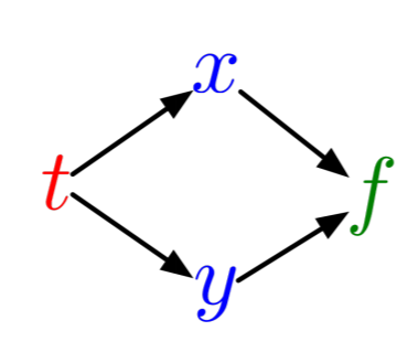
i.e. $t$ directly determines $x$ and $y$ which then determines $f$. To calculate
Assume you've already evaluated $f(t)$. If this has been done, then you've
already had to calculate $x$ and $y$. Thus given the function $f$, we can now
calculate $\frac{df}{dx}$ and $\frac{df}{dy}$, and then calculate $\frac{dx}{dt}$
and $\frac{dy}{dt}$.
Now let's put another layer in the computation. Let's make
$f(x(v(t),w(t)),y(v(t),w(t))$. We can write out the full expression for the
derivative. Notice that even with this additional layer, the
statement we wrote above still holds:
$$\frac{df}{dt} = \frac{df}{dx}\frac{dx}{dt} + \frac{df}{dy}\frac{dy}{dt}$$
So given an evaluation of $f$, we can (still) directly calculate $\frac{df}{dx}$
and $\frac{df}{dy}$. But now, to calculate $\frac{dx}{dt}$ and $\frac{dy}{dt}$,
we do the next step of the chain rule:
$$\frac{dx}{dt} = \frac{dx}{dv}\frac{dv}{dt} + \frac{dx}{dw}\frac{dw}{dt}$$
and similar for $y$. So plug it all in, and you see that our equations will grow
wild if we actually try to plug it in! But it's clear that, to calculate
$$\frac{df}{dt}$$, we can first calculate $\frac{df}{dx}$, and then multiply
that to $\frac{dx}{dt}$. If we had more layers, we could calculate the
*sensitivity* (the derivative) of the output to the last layer, then and then
the sensitivity to the second layer back is the sensitivity of the last layer
multiplied to that, and the third layer back has the sensitivity of the second
layer multiplied to it!
## Logistic Regression Example
To better see this structure, let's write out a simple example. Let our
*forward pass* through our function be:
$$\begin{align}
z &= wx + b\\
y &= \sigma(z)\\
\mathcal{L} &= \frac{1}{2}(y-t)^2\\
\mathcal{R} &= \frac{1}{2}w^2\\
\mathcal{L}_{reg} &= \mathcal{L} + \lambda \mathcal{R}\end{align}$$
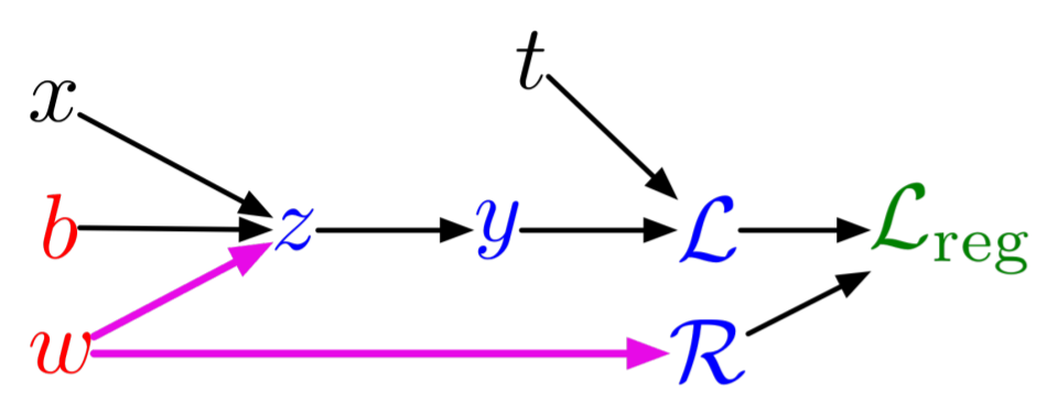
The formulation of the program here is called a *Wengert list, tape, or graph*.
In this, $x$ and $t$ are inputs, $b$ and $W$ are parameters, $z$, $y$, $\mathcal{L}$,
and $\mathcal{R}$ are intermediates, and $\mathcal{L}_{reg}$ is our output.
This is a simple univariate logistic regression model. To do logistic regression,
we wish to find the parameters $w$ and $b$ which minimize the distance of
$\mathcal{L}_{reg}$ from a desired output, which is done by computing derivatives.
Let's calculate the derivatives with respect to each quantity in reverse order.
If our program is $f(x) = \mathcal{L}_{reg}$, then we have that
$$\frac{df}{\mathcal{L}_{reg}} = 1$$
as the derivatives of the last layer. To computerize our notation, let's write
$$\overline{\mathcal{L}_{reg}} = \frac{df}{\mathcal{L}_{reg}}$$
for our computed values. For the derivatives of the second to last layer, we have that:
$$\begin{align}
\overline{\mathcal{R}} &= \frac{df}{\mathcal{L}_{reg}} \frac{d\mathcal{L}_{reg}}{\mathcal{R}}\\
&= \overline{\mathcal{L}_{reg}} \lambda \end{align}$$
$$\begin{align}
\overline{\mathcal{L}} &= \frac{df}{\mathcal{L}_{reg}} \frac{d\mathcal{L}_{reg}}{\mathcal{L}}\\
&= \overline{\mathcal{L}_{reg}} \end{align}$$
This was our observation from before that the derivative of the second layer is
the partial derivative of the current values times the sensitivity of the final
layer. And then we keep multiplying, so now for our next layer we have that:
$$\begin{align}
\overline{y} &= \overline{\mathcal{L}} \frac{d\mathcal{L}}{dy}\\
&= \overline{\mathcal{L}} (y-t) \end{align}$$
And notice that the chain rule holds since $\overline{\mathcal{L}}$ implicitly
already has the multiplication by $\overline{\mathcal{L}_{reg}}$ inside of it.
Then the next layer is:
$$\begin{align}
\frac{df}{z} &= \overline{y} \frac{dy}{dz}\\
&= \overline{y} \sigma^\prime(z) \end{align}$$
Then the next layer. Notice that here, by the chain rule on $w$ we have that:
$$\begin{align}
\overline{w} &= \overline{z} \frac{\partial z}{\partial w} + \overline{\mathcal{R}} \frac{d \mathcal{R}}{dw}\\
&= \overline{z} x + \overline{\mathcal{R}} w\end{align}$$
$$\begin{align}
\overline{b} &= \overline{z} \frac{\partial z}{\partial b}\\
&= \overline{z} \end{align}$$
This completely calculates all derivatives. In conclusion, the rule is:
- You sum terms from each outward arrow
- Each arrow has the derivative term of the end times the partial of the
current term.
- Recurse backwards to build simple linear combination expressions.
### Quick note
We started this derivation with
$$\frac{df}{\mathcal{L}_{reg}} = 1$$
and we then get out $\nabla f(x)$, but from our discussion before this is simply
`[1]' J`. Thus while we have a (flaky) justification for making this value `1`,
it's really just the choice of $v$! Thus doing
$$\frac{df}{\mathcal{L}_{reg}} = v$$
will make this process compute $v^T J$ for this $f$.
## Backpropogation of a Neural Network
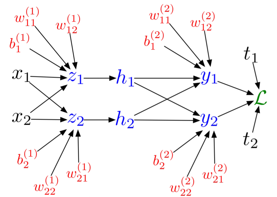
Now let's look at backpropgation of a deep neural network. Before getting to it
in the linear algebraic sense, let's write everything in terms of scalars. This
means we can write a simple neural network as:
$$\begin{align}
z_i &= \sum_j W_{ij}^1 x_j + b_i^1\\
h_i &= \sigma(z_i)\\
y_i &= \sum_j W_{ij}^2 h_j + b_i^2\\
\mathcal{L} &= \frac{1}{2} \sum_k \left(y_k - t_k \right)^2 \end{align}$$
where I have chosen the L2 loss function. This is visualized by the computational
graph:
Then we can do the same process as before to get:
$$\begin{align}
\overline{\mathcal{L}} &= 1\\
\overline{y_i} &= \overline{\mathcal{L}} (y_i - t_i)\\
\overline{w_{ij}^2} &= \overline{y_i} h_j\\
\overline{b_i^2} &= \overline{y_i}\\
\overline{h_i} &= \sum_k (\overline{y_k}w_{ki}^2)\\
\overline{z_i} &= \overline{h_i}\sigma^\prime(z_i)\\
\overline{w_{ij}^1} &= \overline{z_i} x_j\\
\overline{b_i^1} &= \overline{z_i}\end{align}$$
just by examining the computation graph. Now let's write this in linear algebraic
form.
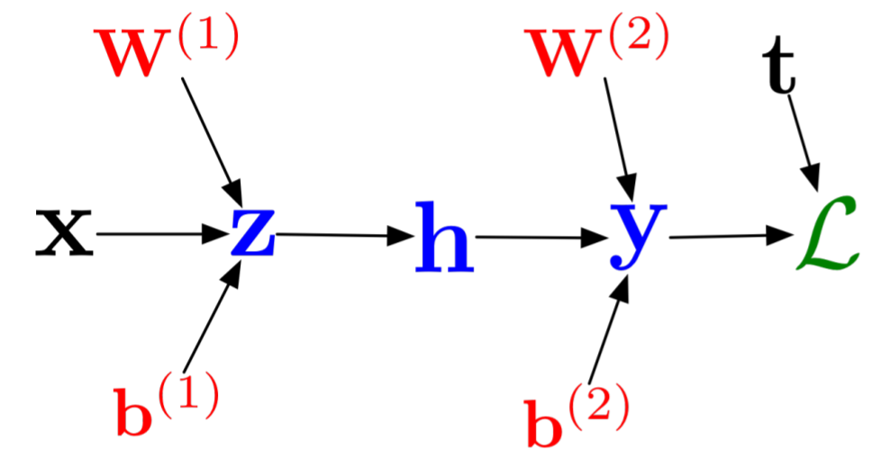
The forward pass for this simple neural network was:
$$\begin{align}
z &= W_1 x + b_1\\
h &= \sigma(z)\\
y &= W_2 h + b_2\\
\mathcal{L} = \frac{1}{2} \Vert y-t \Vert^2 \end{align}$$