This is an implementation of the following paper:

DAGs with NO TEARS: Continuous Optimization for Structure Learning (NIPS 2018, Spotlight)

Xun Zheng, Bryon Aragam, Pradeep Ravikumar, Eric Xing.

If you find it useful, please consider citing:

@inproceedings{zheng2018dags,
    author = {Zheng, Xun and Aragam, Bryon and Ravikumar, Pradeep and Xing, Eric P.},
    booktitle = {Advances in Neural Information Processing Systems {(NIPS)}},
    title = {{DAGs with NO TEARS: Continuous Optimization for Structure Learning}},
    year = {2018}
}

Check out simple_demo.py for a complete, end-to-end implementation of the NOTEARS algorithm in fewer than 50 lines.

A directed acyclic graphical model (aka Bayesian network) with d nodes defines a distribution of random vector of size d. We are interested in the Bayesian Network Structure Learning (BNSL) problem: given n samples from such distribution, how to estimate the graph G?

A major challenge of BNSL is enforcing the directed acyclic graph (DAG) constraint, which is combinatorial. While existing approaches rely on local heuristics, we introduce a fundamentally different strategy: we formulate it as a purely continuous optimization problem over real matrices that avoids this combinatorial constraint entirely. In other words,

where h is a smooth function whose level set exactly characterizes the space of DAGs.

• Python 3.5+
• (optional) C++11 compiler

• Simple NOTEARS (without l1 regularization)
  • simple_demo.py - the 50-line implementation of simple NOTEARS
  • utils.py - graph simulation, data simulation, and accuracy evaluation
• Full NOTEARS (with l1 regularization)
  • cppext/ - C++ implementation of ProxQN
  • notears.py - the full NOTEARS with live progress monitoring
  • live_demo.ipynb - jupyter notebook for live demo

The simplest way to try out NOTEARS is to run the toy demo:

git clone https://github.com/xunzheng/notears.git
cd notears/
pip install -r requirements.txt
python simple_demo.py

This runs the 50-line version of NOTEARS without l1-regularization on a randomly generated 10-node Erdos-Renyi graph. Since the problem size is small, it will only take a few seconds.

You should see output like this:

I1026 02:19:54.995781 87863 simple_demo.py:77] Graph: 10 node, avg degree 4, erdos-renyi graph
I1026 02:19:54.995896 87863 simple_demo.py:78] Data: 1000 samples, linear-gauss SEM
I1026 02:19:54.995944 87863 simple_demo.py:81] Simulating graph ...
I1026 02:19:54.996556 87863 simple_demo.py:83] Simulating graph ... Done
I1026 02:19:54.996608 87863 simple_demo.py:86] Simulating data ...
I1026 02:19:54.997485 87863 simple_demo.py:88] Simulating data ... Done
I1026 02:19:54.997534 87863 simple_demo.py:91] Solving equality constrained problem ...
I1026 02:20:00.791475 87863 simple_demo.py:94] Solving equality constrained problem ... Done
I1026 02:20:00.791845 87863 simple_demo.py:99] Accuracy: fdr 0.000000, tpr 1.000000, fpr 0.000000, shd 0, nnz 17

The Proximal Quasi-Newton algorithm is at the core of the full NOTEARS with l1-regularization. Hence for efficiency concerns it is implemented in a C++ module cppext using Eigen.

To install cppext, download Eigen submodule and compile the extension:

git submodule update --init --recursive
cd cppext/
python setup.py install
cd .. 

The code comes with a Jupyter notebook that runs a live demo. This allows you to monitor the progress as the algorithm runs. Type

jupyter notebook

and click open live_demo.ipynb in the browser. Select Kernel --> Restart & Run All.

(TODO: gif)

• Ground truth: d = 20 nodes, 2d = 40 expected edges.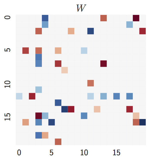

  

• Estimate with n = 1000 samples: lambda = 0, lambda = 0.1, and FGS (baseline).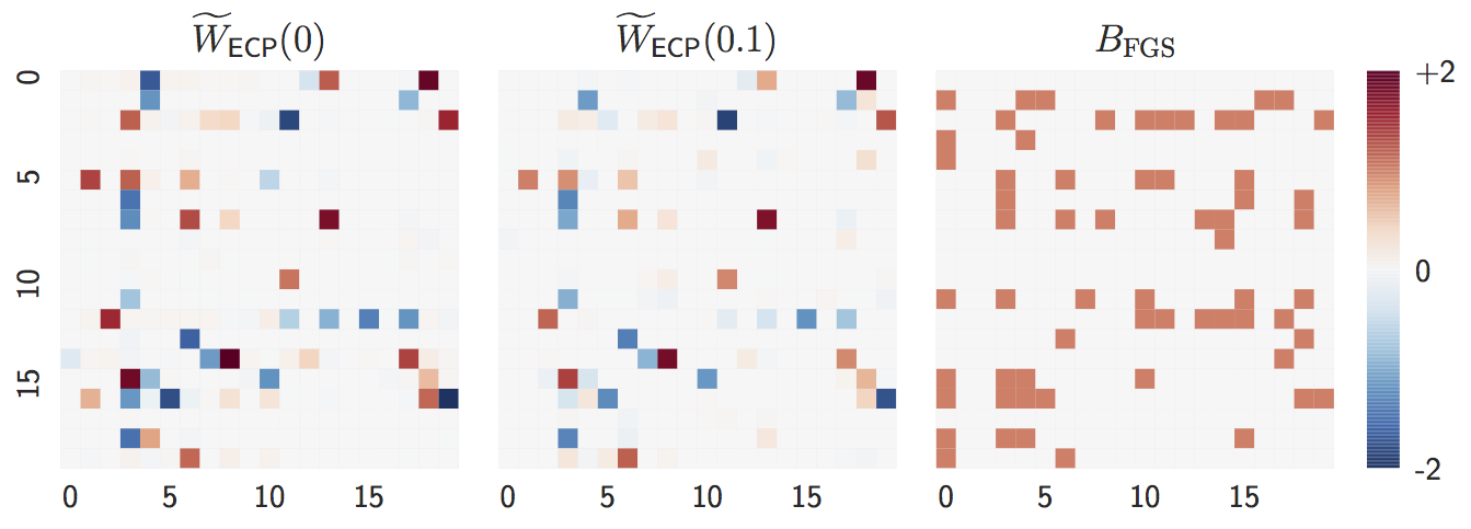

  

  Both lambda = 0 and lambda = 0.1 are close to the ground truth graph when n is large.

• Estimate with n = 20 samples: lambda = 0, lambda = 0.1, and FGS (baseline).

  

  When n is small, lambda = 0 perform worse while lambda = 0.1 remains accurate, showing the advantage of L1-regularization.

• Ground truth: d = 20 nodes, 4d = 80 expected edges.

  

  The degree distribution is significantly different from the Erdos-Renyi graph. One nice property of our method is that it is agnostic about the graph structure.

• Estimate with n = 1000 samples: lambda = 0, lambda = 0.1, and FGS (baseline).

  

  The observation is similar to Erdos-Renyi graph: both lambda = 0 and lambda = 0.1 accurately estimates the ground truth when n is large.

• Estimate with n = 20 samples: lambda = 0, lambda = 0.1, and FGS (baseline).

  

  Similarly, lambda = 0 suffers from small n while lambda = 0.1 remains accurate, showing the advantage of L1-regularization.

• Python: https://github.com/jmoss20/notears