# DAGs with NO TEARS :no_entry_sign::droplet:
**[Update 12/8/22]** Interested in faster and more accurate structure learning? See our new [DAGMA](https://github.com/kevinsbello/dagma) library from [NeurIPS 2022](https://arxiv.org/abs/2209.08037).
This is an implementation of the following papers:
[1] Zheng, X., Aragam, B., Ravikumar, P., & Xing, E. P. (2018). [DAGs with NO TEARS: Continuous optimization for structure learning](https://arxiv.org/abs/1803.01422) ([NeurIPS 2018](https://nips.cc/Conferences/2018/), Spotlight).
[2] Zheng, X., Dan, C., Aragam, B., Ravikumar, P., & Xing, E. P. (2020). [Learning
sparse nonparametric DAGs](https://arxiv.org/abs/1909.13189) ([AISTATS 2020](https://aistats.org/), to appear).
If you find this code useful, please consider citing:
```
@inproceedings{zheng2018dags,
author = {Zheng, Xun and Aragam, Bryon and Ravikumar, Pradeep and Xing, Eric P.},
booktitle = {Advances in Neural Information Processing Systems},
title = {{DAGs with NO TEARS: Continuous Optimization for Structure Learning}},
year = {2018}
}
```
```
@inproceedings{zheng2020learning,
author = {Zheng, Xun and Dan, Chen and Aragam, Bryon and Ravikumar, Pradeep and Xing, Eric P.},
booktitle = {International Conference on Artificial Intelligence and Statistics},
title = {{Learning sparse nonparametric DAGs}},
year = {2020}
}
```
## tl;dr Structure learning in <60 lines
Check out [`linear.py`](notears/linear.py) for a complete, end-to-end implementation of the NOTEARS algorithm in fewer than **60 lines**.
This includes L2, Logistic, and Poisson loss functions with L1 penalty.
## Introduction
A directed acyclic graphical model (aka Bayesian network) with `d` nodes defines a
distribution of random vector of size `d`.
We are interested in the Bayesian Network Structure Learning (BNSL) problem:
given `n` samples from such distribution, how to estimate the graph `G`?
A major challenge of BNSL is enforcing the directed acyclic graph (DAG)
constraint, which is **combinatorial**.
While existing approaches rely on local heuristics,
we introduce a fundamentally different strategy: we formulate it as a purely
**continuous** optimization problem over real matrices that avoids this
combinatorial constraint entirely.
In other words,
 where `h` is a *smooth* function whose level set exactly characterizes the
space of DAGs.
## Requirements
- Python 3.6+
- `numpy`
- `scipy`
- `python-igraph`: Install [igraph C core](https://igraph.org/c/) and `pkg-config` first.
- `torch`: Optional, only used for nonlinear model.
## Contents (New version)
- `linear.py` - the 60-line implementation of NOTEARS with l1 regularization for various losses
- `nonlinear.py` - nonlinear NOTEARS using MLP or basis expansion
- `locally_connected.py` - special layer structure used for MLP
- `lbfgsb_scipy.py` - wrapper for scipy's LBFGS-B
- `utils.py` - graph simulation, data simulation, and accuracy evaluation
## Running a simple demo
The simplest way to try out NOTEARS is to run a simple example:
```bash
$ git clone https://github.com/xunzheng/notears.git
$ cd notears/
$ python notears/linear.py
```
This runs the l1-regularized NOTEARS on a randomly generated 20-node Erdos-Renyi graph with 100 samples.
Within a few seconds, you should see output like this:
```
{'fdr': 0.0, 'tpr': 1.0, 'fpr': 0.0, 'shd': 0, 'nnz': 20}
```
The data, ground truth graph, and the estimate will be stored in `X.csv`, `W_true.csv`, and `W_est.csv`.
## Running as a command
Alternatively, if you have a CSV data file `X.csv`, you can install the package and run the algorithm as a command:
```bash
$ pip install git+git://github.com/xunzheng/notears
$ notears_linear X.csv
```
The output graph will be stored in `W_est.csv`.
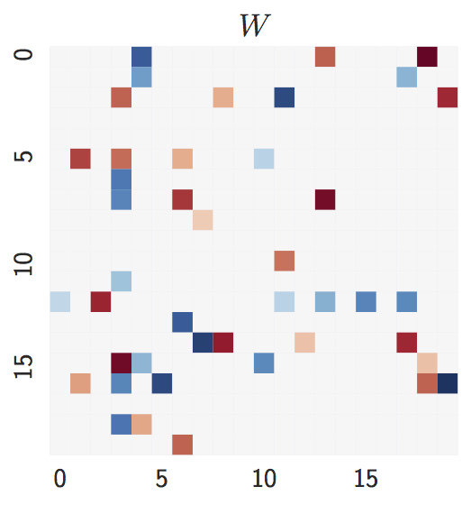
## Examples: Erdos-Renyi graph
- Ground truth: `d = 20` nodes, `2d = 40` expected edges.
where `h` is a *smooth* function whose level set exactly characterizes the
space of DAGs.
## Requirements
- Python 3.6+
- `numpy`
- `scipy`
- `python-igraph`: Install [igraph C core](https://igraph.org/c/) and `pkg-config` first.
- `torch`: Optional, only used for nonlinear model.
## Contents (New version)
- `linear.py` - the 60-line implementation of NOTEARS with l1 regularization for various losses
- `nonlinear.py` - nonlinear NOTEARS using MLP or basis expansion
- `locally_connected.py` - special layer structure used for MLP
- `lbfgsb_scipy.py` - wrapper for scipy's LBFGS-B
- `utils.py` - graph simulation, data simulation, and accuracy evaluation
## Running a simple demo
The simplest way to try out NOTEARS is to run a simple example:
```bash
$ git clone https://github.com/xunzheng/notears.git
$ cd notears/
$ python notears/linear.py
```
This runs the l1-regularized NOTEARS on a randomly generated 20-node Erdos-Renyi graph with 100 samples.
Within a few seconds, you should see output like this:
```
{'fdr': 0.0, 'tpr': 1.0, 'fpr': 0.0, 'shd': 0, 'nnz': 20}
```
The data, ground truth graph, and the estimate will be stored in `X.csv`, `W_true.csv`, and `W_est.csv`.
## Running as a command
Alternatively, if you have a CSV data file `X.csv`, you can install the package and run the algorithm as a command:
```bash
$ pip install git+git://github.com/xunzheng/notears
$ notears_linear X.csv
```
The output graph will be stored in `W_est.csv`.
## Examples: Erdos-Renyi graph
- Ground truth: `d = 20` nodes, `2d = 40` expected edges.
 - Estimate with `n = 1000` samples:
`lambda = 0`, `lambda = 0.1`, and `FGS` (baseline).
- Estimate with `n = 1000` samples:
`lambda = 0`, `lambda = 0.1`, and `FGS` (baseline).
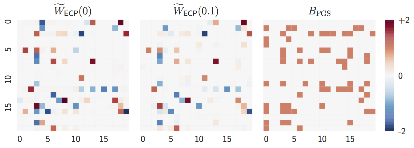 Both `lambda = 0` and `lambda = 0.1` are close to the ground truth graph
when `n` is large.
- Estimate with `n = 20` samples:
`lambda = 0`, `lambda = 0.1`, and `FGS` (baseline).
Both `lambda = 0` and `lambda = 0.1` are close to the ground truth graph
when `n` is large.
- Estimate with `n = 20` samples:
`lambda = 0`, `lambda = 0.1`, and `FGS` (baseline).
 When `n` is small, `lambda = 0` perform worse while
`lambda = 0.1` remains accurate, showing the advantage of L1-regularization.
## Examples: Scale-free graph
- Ground truth: `d = 20` nodes, `4d = 80` expected edges.
When `n` is small, `lambda = 0` perform worse while
`lambda = 0.1` remains accurate, showing the advantage of L1-regularization.
## Examples: Scale-free graph
- Ground truth: `d = 20` nodes, `4d = 80` expected edges.
 The degree distribution is significantly different from the Erdos-Renyi graph.
One nice property of our method is that it is agnostic about the
graph structure.
- Estimate with `n = 1000` samples:
`lambda = 0`, `lambda = 0.1`, and `FGS` (baseline).
The degree distribution is significantly different from the Erdos-Renyi graph.
One nice property of our method is that it is agnostic about the
graph structure.
- Estimate with `n = 1000` samples:
`lambda = 0`, `lambda = 0.1`, and `FGS` (baseline).
 The observation is similar to Erdos-Renyi graph:
both `lambda = 0` and `lambda = 0.1` accurately estimates the ground truth
when `n` is large.
- Estimate with `n = 20` samples:
`lambda = 0`, `lambda = 0.1`, and `FGS` (baseline).
The observation is similar to Erdos-Renyi graph:
both `lambda = 0` and `lambda = 0.1` accurately estimates the ground truth
when `n` is large.
- Estimate with `n = 20` samples:
`lambda = 0`, `lambda = 0.1`, and `FGS` (baseline).
 Similarly, `lambda = 0` suffers from small `n` while
`lambda = 0.1` remains accurate, showing the advantage of L1-regularization.
## Other implementations
- Python: https://github.com/jmoss20/notears
- Tensorflow with Python: https://github.com/ignavier/notears-tensorflow
Similarly, `lambda = 0` suffers from small `n` while
`lambda = 0.1` remains accurate, showing the advantage of L1-regularization.
## Other implementations
- Python: https://github.com/jmoss20/notears
- Tensorflow with Python: https://github.com/ignavier/notears-tensorflow